


Introduction
Machine Learning pipelines are about continuous learning and striving for the highest accuracy. As Data Scientists, our quest for progress is unceasing, and we constantly seek time-saving tips and tricks to advance our work. It’s in this pursuit of efficiency that low-code tools have found their place in the toolkit of data scientists. These tools offer a gateway to harness the potential of external features and data, providing a significant boost to the creation of machine learning pipelines.
This article was published as a part of the Data Science Blogathon.
Table of contents
In this article, we’ll explore two major scenarios for integrating external features and data into your machine learning pipelines.
Final Improvement of a Polished ML Pipelines
The first scenario involves the final improvement of already polished pipelines, aiming to answer the crucial question: Can external data sources and features push the accuracy envelope even further? However, there’s a caveat to this approach: the existing model architecture and hyperparameters may not be the best fit for the new feature set, potentially requiring an extra step back for model tuning.
Low-code Initial Feature Engineering – Add Relevant External Features @start
The second scenario focuses on low-code initial feature engineering, allowing you to add relevant external features right from the start. This approach is a time-saver in feature search and engineering. Still, it’s essential to ensure these external features are optimally aligned with the specific task and target model architecture. As you delve into external data for machine learning pipelines, remember that while more features can be beneficial, they should be chosen carefully to avoid dimensionality increase and model overfitting. Throughout this article, we’ll explore these scenarios in-depth, equipping you with the knowledge and skills to make the most of external data sources in your machine learning endeavors.
Let’s Get Started
In this guide, we’ll go with Scenario #1.
Let’s resolve such a task: TPS January 2022, SMAPE as a target metric.
And get the best open notebook for improvement.
To search for useful external data, we’ll use:
Upgini – Low-code Feature search and enrichment python library for supervised machine learning applications.
Packages
Let’s install and import the packages that we will need.
%pip install -Uq upgini import pandas as pd
import numpy as np
import pickle
import itertools
import gc
import math
import matplotlib.pyplot as plt
import dateutil.easter as easter
from datetime import datetime, date, timedelta
from sklearn.preprocessing import StandardScaler, MinMaxScaler
from sklearn.impute import SimpleImputer
from sklearn.model_selection import KFold, GroupKFold, TimeSeriesSplit
from sklearn.linear_model import Ridge
from sklearn.metrics import mean_squared_error
from sklearn.compose import ColumnTransformer
from sklearn.pipeline import make_pipeline
import lightgbm as lgb
import scipy.stats
import osPython Code:
def generate_main_features(df):

    new_df = df[["row_id", "date", "country", "segment", "num_sold"]].copy()

    ## one-hot encoding

    new_df['Rama'] = df.store == 'Rama'

    for country in ['Finland', 'Norway']:

        new_df[country] = df.country == country

    for product in ['Mug', 'Hat']:

        new_df[product] = df['product'] == product


    ## datetime features

    new_df['wd4'] = np.where(df.date.dt.weekday == 4, 1, 0)

    new_df['wd56'] = np.where(df.date.dt.weekday >= 5, 1, 0)


    dayofyear = df.date.dt.dayofyear

    for k in range(1, 3):

        sink = np.sin(dayofyear / 365 * 2 * math.pi * k)

        cosk = np.cos(dayofyear / 365 * 2 * math.pi * k)

        new_df[f'mug_sin{k}'] = sink * new_df['Kaggle Mug']

        new_df[f'mug_cos{k}'] = cosk * new_df['Kaggle Mug']

        new_df[f'hat_sin{k}'] = sink * new_df['Kaggle Hat']

        new_df[f'hat_cos{k}'] = cosk * new_df['Kaggle Hat']

    new_df.drop(columns=['mug_sin1'], inplace=True)

    new_df.drop(columns=['mug_sin2'], inplace=True)


    # special days

    new_df = pd.concat([

        new_df,

        pd.DataFrame({f"dec{d}":(df.date.dt.month == 12) & (df.date.dt.day == d) for d in range(24, 32)}),

        pd.DataFrame({

            f"n-dec{d}": (df.date.dt.month == 12) & (df.date.dt.day == d) & (df.country == 'Norway')

            for d in range(25, 32)

        }),

        pd.DataFrame({

            f"f-jan{d}": (df.date.dt.month == 1) & (df.date.dt.day == d) & (df.country == 'Finland')

            for d in range(1, 15)

        }),

        pd.DataFrame({

            f"n-jan{d}": (df.date.dt.month == 1) & (df.date.dt.day == d) & (df.country == 'Norway')

            for d in range(1, 10)

        }),

        pd.DataFrame({

            f"s-jan{d}": (df.date.dt.month == 1) & (df.date.dt.day == d) & (df.country == 'Sweden')

            for d in range(1, 15)

        })

    ], axis=1)


    # May and June

    new_df = pd.concat([

        new_df,

        pd.DataFrame({

            f"may{d}": (df.date.dt.month == 5) & (df.date.dt.day == d)

            for d in list(range(1, 10))

        }),

        pd.DataFrame({

            f"may{d}": (df.date.dt.month == 5) & (df.date.dt.day == d) & (df.country == 'Norway')

            for d in list(range(18, 26)) + [27]

        }),

        pd.DataFrame({

            f"june{d}": (df.date.dt.month == 6) & (df.date.dt.day == d) & (df.country == 'Sweden')

            for d in list(range(8, 15))

        })

    ], axis=1)


    # Last Wednesday of June

    wed_june_map = {

        2015: pd.Timestamp(('2015-06-24')),

        2016: pd.Timestamp(('2016-06-29')),

        2017: pd.Timestamp(('2017-06-28')),

        2018: pd.Timestamp(('2018-06-27')),

        2019: pd.Timestamp(('2019-06-26'))

    }

    wed_june_date = df.date.dt.year.map(wed_june_map)

    new_df = pd.concat([

        new_df,

        pd.DataFrame({

            f"wed_june{d}": (df.date - wed_june_date == np.timedelta64(d, "D")) & (df.country != 'Norway')

            for d in list(range(-4, 5))

        })

    ], axis=1)


    # First Sunday of November

    sun_nov_map = {

        2015: pd.Timestamp(('2015-11-1')),

        2016: pd.Timestamp(('2016-11-6')),

        2017: pd.Timestamp(('2017-11-5')),

        2018: pd.Timestamp(('2018-11-4')),

        2019: pd.Timestamp(('2019-11-3'))

    }

    sun_nov_date = df.date.dt.year.map(sun_nov_map)

    new_df = pd.concat([

        new_df,

        pd.DataFrame({

            f"sun_nov{d}": (df.date - sun_nov_date == np.timedelta64(d, "D")) & (df.country != 'Norway')

            for d in list(range(0, 9))

        })

    ], axis=1)


    # First half of December (Independence Day of Finland, 6th of December)

    new_df = pd.concat([

        new_df,

        pd.DataFrame({

            f"dec{d}": (df.date.dt.month == 12) & (df.date.dt.day == d) & (df.country == 'Finland')

            for d in list(range(6, 15))

        }

    )], axis=1)


    # Easter

    easter_date = df.date.apply(lambda date: pd.Timestamp(easter.easter(date.year)))

    new_df = pd.concat([

        new_df,

        pd.DataFrame({

            f"easter{d}": (df.date - easter_date == np.timedelta64(d, "D"))

            for d in list(range(-2, 11)) + list(range(40, 48)) + list(range(51, 58))

        }),

        pd.DataFrame({

            f"n_easter{d}": (df.date - easter_date == np.timedelta64(d, "D")) & (df.country == 'Norway')

            for d in list(range(-3, 8)) + list(range(50, 61))

        })

    ], axis=1)


    features_list = [

        f for f in new_df.columns

        if f not in ["row_id", "date", "segment", "country", "num_sold", "Rama"]

    ]

    return new_df, features_list


def get_gdp(row):

    country = 'GDP_' + row.country

    return gdp_df.loc[row.date.year, country]


def get_cci(row):

    country = row.country

    time = f"{row.date.year}-{row.date.month:02d}"

    if country == 'Norway': country = 'Finland'

    return cci_df.loc[country[:3].upper(), time].Value


def generate_extra_features(df, features_list):

    df['gdp'] = np.log(df.apply(get_gdp, axis=1))

    df['cci'] = df.apply(get_cci, axis=1)

    features_list_upd = features_list + ["gdp", "cci"]


    return df, features_list_upd
Final Improvement of Polished Pipeline
The objective here is to maximize the utility of external data sources, leveraging their potential to boost the accuracy of your already refined machine learning pipeline. In this section, we will explore strategies for seamlessly integrating external data sources into a well-structured pipeline, ensuring that the final result is a sophisticated and optimized model capable of delivering superior performance.
Step 1: Let’s take an existing open solution with external data as a baseline
There are already external data in this solution, so improvement shouldn’t be an easy walk ;-):
- GDP statistics per year/country (“gdp-20152019-finland-norway-and-sweden” dataset);
- Consumer Confidence Index per year/month/country (Value field of “oecd-consumer-confidence-index” dataset).
And we want to improve the winning kernel by finding new/better external features.
There are no changes in feature engineering from the original notebook by @ambrosm.
So let’s calculate metrics for the baseline solution. First, read train/test data from csv, combine them in one dataframe and generate features:
input_data_path = "/input"
df, rama_ratio = read_main_data(input_data_path)
# a lot of calendar based features
df, baseline_features = generate_main_features(df)
print(df.shape)
print("Number of features:", len(baseline_features))
df.segment.value_counts()
# features from GDP and CCI
gdp_df, cci_df = read_additional_data(input_data_path)
df, top_solution_features = generate_extra_features(df, baseline_features)
print(df.shape)
set(top_solution_features) - set(baseline_features)
Output:
(32868, 172) Number of features: 166 (32868, 174)
{'cci', 'gdp'}
Define model, cross-validation split and apply cross-validation to estimate model accuracy:
model = Ridge(alpha=0.2, tol=0.00001, max_iter=10000)
cv = KFold(n_splits=5)
top_solution_scores, model_coef = cross_validate(model, df, top_solution_features, rama_ratio, cv=cv)
print("Top solution SMAPE by folds:", top_solution_scores)
print("Top solution avg SMAPE:", sum(top_solution_scores)/len(top_solution_scores))Output:
Top solution SMAPE by folds: [4.239, 4.159, 4.168, 4.293, 4.077]
Top solution avg SMAPE: 4.1872
Now, make the submission file:
submission_path = 'submission_top_solution.csv'
make_submission(model, df, top_solution_features, rama_ratio, submission_path)
The submission scores 4.13 on the public leaderboard and 4.55 on the private leaderboard (first place in the competition). This is our baseline.
Can we improve the first place solution even more? Let’s find out!
Step 2: Find Relevant External Features
In our quest to discover novel features, we turn to Upgini Feature search and enrichment library for supervised machine learning applications. To initiate a search with the Upgini library, you must define so-called search keys – a set of columns to join external data sources. In this competition, we can use the following keys:
- Column date should be used as SearchKey.DATE.;
- Column country (after conversion to ISO-3166 country code) should be used as SearchKey.COUNTRY.
With this set of search keys, our dataset will be matched with different time-specific features (such as weather data, calendar data, financial data, etc.), considering the country where sales happened. Then relevant selection and ranking will be made. As a result, we’ll add new, only relevant features with additional information about specific dates and countries.
from upgini import SearchKey

# here we simply map each country to its ISO-3166 code
country_iso_map = {
    "Finland": "FI",
    "Norway": "NO",
    "Sweden": "SE"
}
df["country_iso"] = df.country.map(country_iso_map)

## define search keys
search_keys = {
    "date": SearchKey.DATE,
    "country_iso": SearchKey.COUNTRY
}
To start the search, we need to initiate a scikit-learn compatible FeaturesEnricher transformer with appropriate search parameters. After that, we can call the fit method features_enricher to start the search.
The ratio between Rama and Mart sales is constant, so we’ll use only Mart sales for feature search and model training:
%%time
from upgini import FeaturesEnricher
from upgini.metadata import CVType, RuntimeParameters

## define X_train / y_train, remove Mart
condition = (df.segment == "train") & (df.Rama == False)
X_train, y_train = df.loc[condition, list(search_keys.keys()) + top_solution_features], df.loc[condition, "num_sold"]

## define Features Enricher
features_enricher = FeaturesEnricher(
    search_keys = search_keys
)
Output:
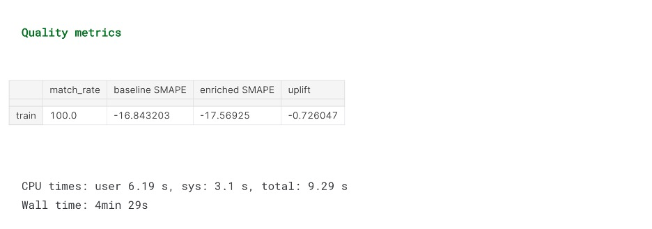
CPU times: user 82 ms, sys: 14.7 ms, total: 96.7 ms Wall time: 4.59 sFeaturesEnricher.fit() has a flag calculate_metrics
For the quick estimation of quality improvement on cross-validation and eval sets. This step is quite similar to sklearn.model_selection.cross_val_score, so you can pass the exact metric with the scoring parameter:
- Built-in scoring functions;
- Custom scorer (in this case – scorer based on SMAPE loss).
And we pass the final Ridge model estimator with parameter, estimator for correct metric calculation, right in search results.
Notice that you should pass X_train as the first argument and y_train as the second argument for, FeaturesEnricher.fit(), just like in scikit-learn.
The step will take around 3.5 minutes
%%time
from sklearn.metrics import make_scorer

## define SMAPE custom scoring function
scorer = make_scorer(smape_loss, greater_is_better=False)
scorer.__name__ = "SMAPE"

## launch fit
features_enricher.fit(X_train, y_train,
                      calculate_metrics = True,
                      scoring = scorer,
                      estimator = model)
Output:
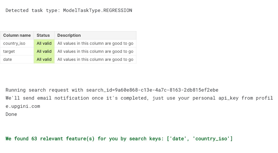
Relevant Features
| feature_name | shap_value | coverage % | type | |
|---|---|---|---|---|
| 0 | Hat | 0.507071 | 100.000000 | NUMERIC |
| 1 | Mug | 0.115800 | 100.000000 | NUMERIC |
| 2 | f_cci_1y_shift_0fa85f6f | 0.088312 | 66.666667 | NUMERIC |
| 3 | mug_cos1 | 0.046179 | 100.000000 | NUMERIC |
| 4 | f_pcpiham_wt_531b4347 | 0.029045 | 100.000000 | NUMERIC |
| 5 | f_cci_6m_shift_653a5999 | 0.022123 | 66.666667 | NUMERIC |
| 6 | f_year_sin1_16137bbf | 0.019437 | 100.000000 | NUMERIC |
| 7 | f_weekend_d0c2211b | 0.014037 | 100.000000 | NUMERIC |
| 8 | f_c2c_fraud_score_5028232e | 0.010249 | 100.000000 | NUMERIC |
| 9 | hat_sin1 | 0.010188 | 100.000000 | NUMERIC |
| 10 | f_pcpihac_ix_16f52c8e | 0.009000 | 100.000000 | NUMERIC |
| 11 | f_credit_default_score_05229fa7 | 0.008933 | 100.000000 | NUMERIC |
| 12 | f_weather_pca_0_94efd18d | 0.007758 | 100.000000 | NUMERIC |
| 13 | f_pcpih_wt_10c16d11 | 0.007703 | 100.000000 | NUMERIC |
| 14 | Norway | 0.007180 | 100.000000 | NUMERIC |
| 15 | wd56 | 0.006366 | 100.000000 | NUMERIC |
| 16 | f_pcpihah_ix_260dd0c8 | 0.006058 | 100.000000 | NUMERIC |
| 17 | f_payment_fraud_score_3cae9c42 | 0.005449 | 100.000000 | NUMERIC |
| 18 | f_cci_diff_1m_shift_fa99295c | 0.004708 | 66.666667 | NUMERIC |
| 19 | f_transaction_fraud_union_score_f9bc093c | 0.003007 | 100.000000 | NUMERIC |
| 20 | f_cci_pca_8_b72fe9f6 | 0.002578 | 100.000000 | NUMERIC |
| 21 | f_holiday_public_7d_before_e3186344 | 0.002564 | 100.000000 | NUMERIC |
| 22 | f_pcpih_ix_c2a9fea0 | 0.002472 | 100.000000 | NUMERIC |
| 23 | f_days_to_election_e6b7c247 | 0.002158 | 100.000000 | NUMERIC |
| 24 | f_pcpir_pc_cp_a_pt_3c2d5a5f | 0.001977 | 100.000000 | NUMERIC |
| 25 | f_holiday_national_7d_before_5ca8fb46 | 0.001935 | 100.000000 | NUMERIC |
| 26 | f_pcpihabt_pc_cp_a_pt_41878919 | 0.001789 | 100.000000 | NUMERIC |
| 27 | f_pcpihao_pc_cp_a_pt_0c75e62a | 0.001649 | 100.000000 | NUMERIC |
| 28 | mug_cos2 | 0.001381 | 100.000000 | NUMERIC |
| 29 | f_cci_1m_shift_8b298796 | 0.001263 | 66.666667 | NUMERIC |
| 30 | f_days_from_election_e1441706 | 0.001253 | 100.000000 | NUMERIC |
| 31 | f_pcpi_pc_cp_a_pt_c1d5fdeb | 0.001235 | 100.000000 | NUMERIC |
| 32 | f_gold_7d_to_1y_1df66550 | 0.001215 | 100.000000 | NUMERIC |
| 33 | f_holiday_code_7d_before_34f02a4f | 0.001169 | 100.000000 | NUMERIC |
| 34 | f_pcpifbt_ix_466ad65e | 0.001150 | 100.000000 | NUMERIC |
| 35 | f_holiday_bank_7d_before_efe82fb3 | 0.001147 | 100.000000 | NUMERIC |
| 36 | f_pcpiec_ix_5dc7bc66 | 0.001098 | 100.000000 | NUMERIC |
| 37 | f_cci_diff_6m_shift_52eb4cfe | 0.001090 | 66.666667 | NUMERIC |
| 38 | f_pcpied_pc_pp_pt_07be13cf | 0.001085 | 100.000000 | NUMERIC |
| 39 | f_pcpihah_wt_aad13a53 | 0.001043 | 100.000000 | NUMERIC |
| 40 | f_PCPIEPCH_47b21aec | 0.001013 | 100.000000 | NUMERIC |
| 41 | f_year_sin2_46dc3051 | 0.000979 | 100.000000 | NUMERIC |
| 42 | f_pcpio_ix_e60d7742 | 0.000933 | 100.000000 | NUMERIC |
| 43 | f_year_cos1_cd165f8c | 0.000922 | 100.000000 | NUMERIC |
| 44 | f_pcpif_pc_cp_a_pt_507a914e | 0.000915 | 100.000000 | NUMERIC |
| 45 | gdp | 0.000882 | 100.000000 | NUMERIC |
| 46 | f_pcpir_ix_90fbe7c2 | 0.000867 | 100.000000 | NUMERIC |
| 47 | Finland | 0.000851 | 100.000000 | NUMERIC |
| 48 | f_year_sin10_927d1cbc | 0.000821 | 100.000000 | NUMERIC |
| 49 | f_pcpihat_pc_cp_a_pt_803f3022 | 0.000787 | 100.000000 | NUMERIC |
| 50 | f_days_to_holiday_5ce1a653 | 0.000755 | 100.000000 | NUMERIC |
| 51 | f_cpi_pca_6_00674469 | 0.000713 | 100.000000 | NUMERIC |
| 52 | f_year_cos2_2d8bf75c | 0.000683 | 100.000000 | NUMERIC |
| 53 | f_week_sin1_a71d22f6 | 0.000673 | 100.000000 | NUMERIC |
| 54 | f_days_from_holiday_fbad7b66 | 0.000658 | 100.000000 | NUMERIC |
| 55 | f_BCA_1y_shift_bcc8c904 | 0.000637 | 100.000000 | NUMERIC |
| 56 | f_us_days_from_election_1658c931 | 0.000611 | 100.000000 | NUMERIC |
| 57 | f_cpi_pca_2_3c36cd6c | 0.000597 | 100.000000 | NUMERIC |
| 58 | f_usd_eb23e09d | 0.000591 | 100.000000 | NUMERIC |
| 59 | f_dow_jones_89547e1d | 0.000578 | 100.000000 | NUMERIC |
Exploring the Features
We’ve got 60+ relevant features, which might improve the model’s accuracy. Ranked by SHAP values.
Initial features from the search dataset will also be checked for relevancy, so you don’t need an extra feature selection step.
SMAPE uplift after enrichment with all of the new external features is negative – as it doesn’t make sense to use ALL of them for the linear Ridge model.
Let’s enrich the initial feature space with only the TOP-3 most important features.
Generally, it’s a bad idea to put a lot of features with unknown structure (and possibly high pairwise correlation) into a linear model, like Ridge or Lasso without careful selection and pre-processing.
This step will take around 2 minutes
%%time

## call transform and enrich dataset with TOP-3 features only
df_enriched = features_enricher.transform(df, max_features=3, keep_input = True)

## put top-3 new external features names into selected features list
enricher_features = [
    f for f in features_enricher.get_features_info().feature_name.values
    if f not in list(search_keys.keys()) + top_solution_features
]
best_enricher_features = enricher_features[:3]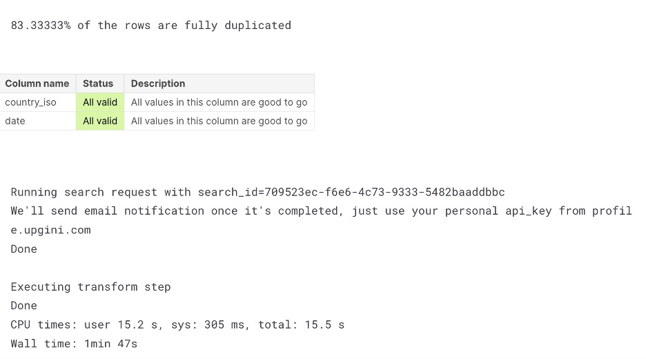
Step 3: Submit and Calculate the Final Leaderboard Progress
Let’s estimate model quality and make a submission file:
#same cross-validation split and model estimator as for baseline notebook in #1 Part
upgini_scores, model_coef = cross_validate(
    model, df_enriched,
    top_solution_features + best_enricher_features,
    rama_ratio, cv=cv
)
print("Top solution SMAPE by folds:", top_solution_scores)
print("Upgini SMAPE by folds:", upgini_scores)
print("Top solution avg SMAPE:", sum(top_solution_scores)/len(top_solution_scores))
print("Upgini avg SMAPE:", sum(upgini_scores)/len(upgini_scores))
Output:
Top solution SMAPE by folds: [4.239, 4.159, 4.168, 4.293, 4.077]
Upgini SMAPE by folds: [4.26, 4.129, 4.144, 4.258, 4.051]
Top solution avg SMAPE: 4.1872
Upgini avg SMAPE: 4.1684
Make a submission file:
submission_path = 'submission.csv'
make_submission(
    model, df_enriched,
    top_solution_features + best_enricher_features,
    rama_ratio, submission_path)
This submission scores 4.095 on public LB and 4.50 on private LB.
Just to remind you – the baseline TOP-1 solution had 4.13 on public LB and 4.55 on private LB (with 2 external data sources already).
We’ve got a consistent improvement both in public and private parts of LB!
Relevant External Features & Data Sources
Leader board accuracy improved from enrichment with 3 new external features:
- f_cci_1y_shift_0fa85f6f – Consumer Confidence Index with 1 year lag. It’s a Consumer Confidence Index value derivative for Finland and Sweden (CCI is unavailable for Norway). CCI as a feature already has been introduced in the baseline notebook, but as a raw CCI index value with scaling on the data prep step.
- f_pcpiham_wt_531b4347 – Consumer Price index for Health group of products & services. In general, Consumer price indexes are index numbers that measure changes in the prices of goods and services purchased or otherwise acquired by households, which households use directly or indirectly to satisfy their needs and wants.
So it has a lot of information about inflation in a specific country and for a specific types of services and goods.
It’s been updated by the Organisation for Economic Cooperation and Development (OECD) every month. - f_cci_6m_shift_653a5999 – Consumer Confidence Index with 6 months lag.
Conclusion
When solving machine learning pipelines task, many data scientists forget that accuracy can be improved by implementing useful external data. Searching for external data can make the accuracy of your machine learning pipeline better, more accurate, and thus make you more money. I showed you how to find useful external data for minutes in this article.
Key takeaways of the article:
- The article contains a description with python code of the way of developing of machine learning model with the best accuracy;
- After reading the article, one can easily improve its ML model with external data;
- The article contains an example of the real syntax of using the upgini python library;
- Moreover, there is a list of real external data contained in upgini database for ML models that improves existing solution for ML tasks.
I hope you liked my article on machine learning pipelines and if you have any feedback or concerns, share with me in the comments below.
Frequently Asked Questions
Q1. What are ML data pipelines?
A. Machine Learning (ML) data pipelines are structured processes for managing and preparing data for use in machine learning models. These pipelines encompass data collection, cleaning, transformation, and feature engineering steps to ensure high-quality data crucial for accurate model training and predictions.
Q2. What is the difference between internal and external data models?
A.Internal data models are designed for an organization’s internal use, tailored to its specific needs, and typically not exposed to external parties. In contrast, external data models are meant to be accessible and interacted with by external users, such as customers, partners, or the public, often through APIs or data sharing.
Q3. What is the difference between data pipeline and ML pipeline?
A. Data pipelines focus on data collection, preprocessing, and storage. They ensure data quality and consistency. ML pipelines, on the other hand, include data processing steps along with model training and deployment stages, encompassing the end-to-end process of creating and deploying machine learning models.
Q4. How do you create a machine learning data pipeline?
A. To create a machine learning data pipeline, follow these steps:
(a) Collect relevant data from various sources.
(b) Preprocess the data, including cleaning, transformation, and handling missing values.
(c) Perform feature engineering to create meaningful model features.
(d) Split the data into training and testing sets.
(e) Choose, train, and evaluate machine learning models.
(f) Deploy the trained model for making predictions.
(g) Continuously monitor and maintain the pipeline for optimal performance and updates.
The media shown in this article is not owned by Analytics Vidhya and is used at the Author’s discretion.