This article was published as a part of the Data Science Blogathon
Introduction- Hyperparameters in a neural network
A deep neural network consists of multiple layers: an input layer, one or multiple hidden layers, and an output layer. In order to develop any deep learning model, one must decide on the most optimal values of a number of hyperparameters such as activation functions, batch size, and learning rate amongst others so as to be able to fine-tune each of these layers.
A hyperparameter controls the learning process and therefore their values directly impact other parameters of the model such as weights and biases which consequently impacts how well our model performs. The accuracy of any machine learning model is most often improved by fine-tuning these hyperparameters. It, therefore, becomes imperative for a machine learning researcher to understand these hyperparameters well.
In this article, we would dig deep into some of the above-mentioned hyperparameters and look at how changing them impacts the model performance.
Dataset
We have considered the Pima Indian Diabetes Dataset here that contains information on 768 women from a population near Phoenix, Arizona, USA. The dependent variable here is Diabetes. 268 out of 768 women belong to the ‘positive’ class while the rest 500 belong to the ‘negative’ class. There are 8 attributes in the dataset – pregnancies, OGTT(Oral Glucose Tolerance Test), blood pressure, skin thickness, insulin, BMI(Body Mass Index), age, and pedigree diabetes function.
Structure of the Network
The structure of the neural network we used consisted of an 8-node input layer. This was followed by the first hidden layer that had 12 nodes. The second hidden layer had 8 nodes, all of which were then connected to a single node in the output layer. The output layer was for producing a binary output value with a sigmoid activation function since we were dealing with a binary classification problem.
Experiments
The following table shows the settings of the different experiments we carried out in order to study the effect of the hyperparameters on our model performance.

Effect of Batch Size
The gradient descent technique is used to train neural networks. In this technique, the estimate of the error (difference between actual and predicted variables) based on a subset of the training dataset is used to update the weights in every iteration. Batch size is defined as the number of examples that are used from the training dataset for estimating the error gradient and is an important hyperparameter that influences the dynamics of the learning algorithm. In mini-batch gradient descent, the batch size is set to more than one and less than the total number of examples in the training dataset.
In Python, the batch size can be specified while training the model as follows:
history = model.fit(X_train,y_train,validation_data=(X_test,y_test),epochs=NB_EPOCHS,batch_size=BATCH_SIZE,verbose=0,shuffle=False)
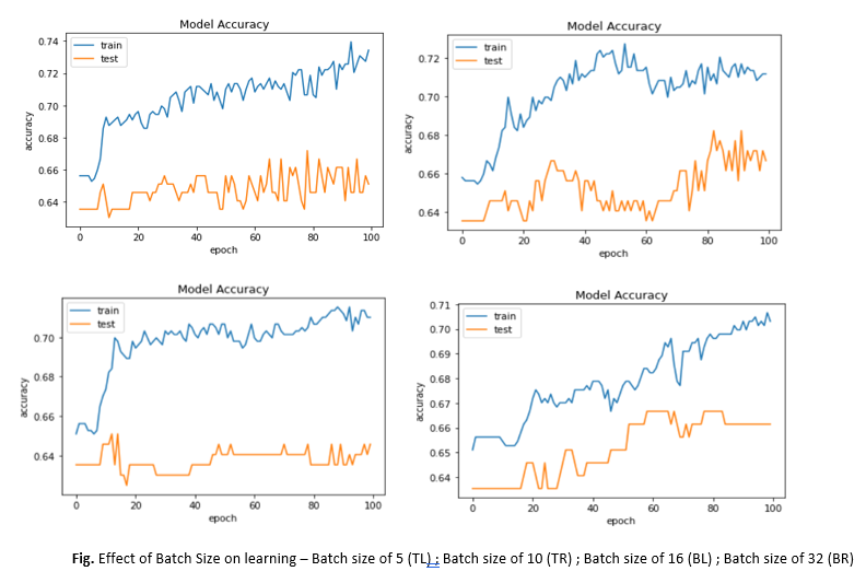
The above plots show the classification accuracy of models with our train and test datasets with different batch sizes when using mini-batch gradient descent.
The plots show that –
- Small batch sizes of 5 and 10 result generally in rapid learning (achieving accuracies on training dataset above 0.72 within 100 epochs) but a volatile learning process with higher variance in the classification accuracy.
- Larger batch sizes of 16 and 32 slow down the learning process (achieving lower accuracies (<0.72) on training dataset within 100 epochs) but the final stages (between 80 to 100 epochs) result in a more stable model exemplified by lower variance in classification accuracy.
Effect of Activation Functions
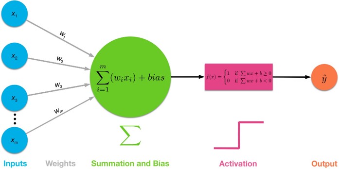
An activation function in a neural network transforms the weighted sum of the inputs into an output from a node in a layer of the network. If an activation function is not used, the neural networks become just a linear regression model as these functions enable the non-linear transformation of the inputs making them capable to learn and perform more complex tasks. There are several commonly used non-linear activation functions like sigmoid, tanh, and ReLU.
In Python, the activation function for each hidden layer can be specified while building the model using Keras as follows:
from keras.models import Sequential
model = Sequential()
model.add(Dense(12, input_dim=8, activation='relu',kernel_initializer='uniform'))
model.add(Dense(8, activation='relu',kernel_initializer='uniform'))
model.add(Dense(1,activation='sigmoid' ,kernel_initializer='uniform'))
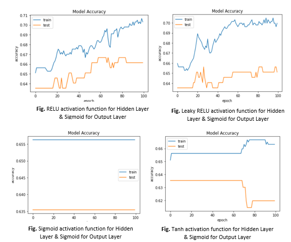
The above plots show the classification accuracy of models with our train and test datasets with different activation functions in the hidden layers.
- With sigmoid and tanh activation functions in the hidden layer, we observe from the plots that almost no learning takes place in the epochs. Both sigmoid and tanh activation functions are known to suffer from vanishing gradient problem, which could be a reason behind observing this behavior while using them in the hidden layer.
- Since activation functions like ReLU and leaky ReLU are not challenged by the vanishing gradient problem, we observed active learning happening through the epochs while using them in the hidden layer.
Effect of Optimizers
While training a deep learning model, the weights and biases associated with each node of a layer are updated at every iteration with the objective of minimizing the loss function. This adjustment of weights is enabled by algorithms like stochastic gradient descent which are also known by the name of optimizers.
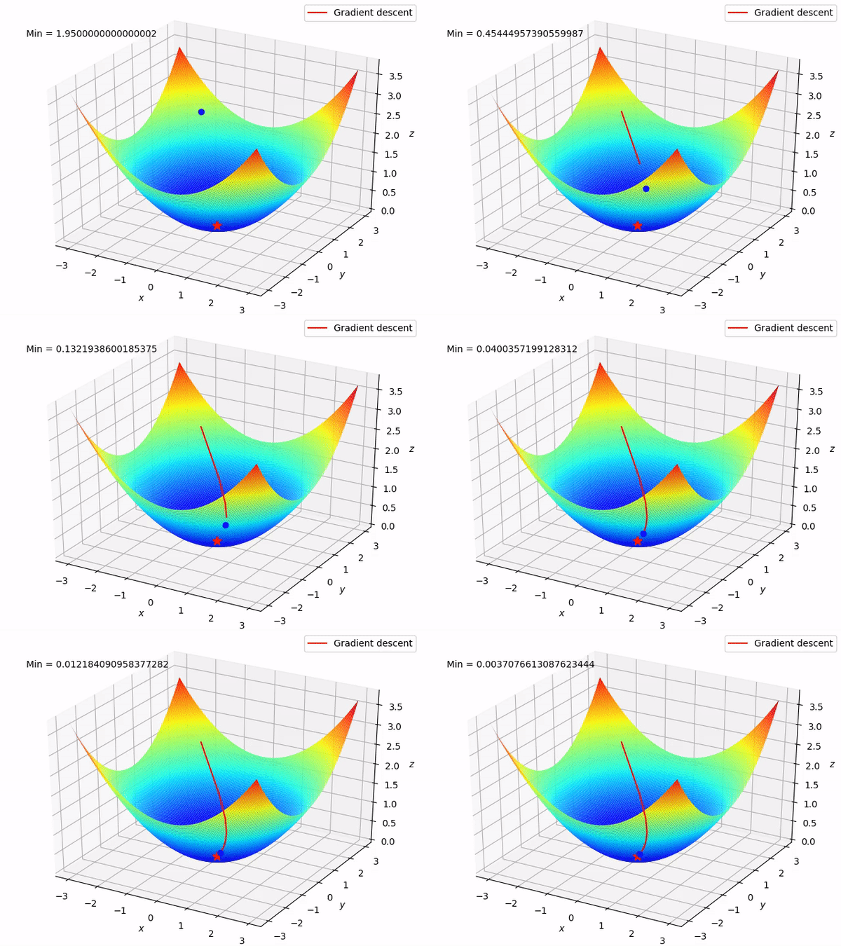
Other algorithms like adaptive learning rate optimizers adjust the learning rate throughout training in response to the performance of the model. Perhaps the simplest implementation is to make the learning rate smaller once the performance of the model plateaus, such as by decreasing the learning rate by a factor of two or an order of magnitude. Although no single method works best on all problems, there are many adaptive learning rate methods that have proven to be robust over many types of neural network architectures and problem types. They are AdaGrad, RMSProp, Adam, AdaMax, and all maintain and adapt learning rates for each of the weights in the model.
In Python, we can specify the type of optimizer while building the model in Keras as follows :
from keras import optimizers
sgd = optimizers.SGD(lr=0.001)
rmsprop = optimizers.RMSprop(lr=0.001)
adagrad = optimizers.Adagrad(lr=0.001)
adam = optimizers.Adam(lr=0.001)
adamax = optimizers.Adamax(lr=0.001)
# Compile the model
model.compile(loss='binary_crossentropy',   optimizer=rmsprop, metrics=['accuracy'])
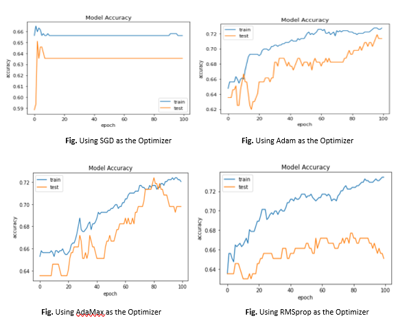
From the plots given above, we can see that
- SGD with a learning rate of 0.001 doesn’t achieve an accuracy of 0.7 on the training dataset even with 100 epochs while RMSprop, AdaMax, and Adam effectively learn the problem and achieve this accuracy on the training dataset much before 100 epochs.
- RMSprop, AdaMax, and Adam are adaptive learning rate optimizers where the learning rates for each of the weights in the model can be adapted based on the response to the model performance.
Conclusion
The effects of various hyperparameter configurations on the performance of a deep learning model for diabetes prediction were investigated in this study.
- Large batch sizes were observed to slow down the learning process but produce a more stable model (as exemplified by lower variance in classification accuracy) as compared to smaller batch sizes.
- Using activation functions like ReLU and leaky ReLU in the hidden layer helped in resolving the vanishing gradient problem as observed while using sigmoid and tanh activation functions.
- Adaptive learning rate optimizers like RMSprop, AdaMax, and Adam were seen to effectively learn and achieve a higher accuracy faster as compared to when using stochastic gradient descent with the same learning rate (0.001).
The media shown in this article is not owned by Analytics Vidhya and is used at the Author’s discretion.


