This article was published as a part of the Data Science Blogathon.
Introduction
A loan default occurs when a borrower takes money from a bank and does not repay the loan. People often default on loans due to various reasons. Borrowers who default on loans not only damage their credit but also risk being sued and having their wages garnished. Let’s take a look at the types of defaults that happen and understand the various reasons why people take loans and learn how predicting loan default will work.

Source: Pexels.com
Types of Default
A secured debt default can occur, such as with a mortgage loan secured by a property or a business loan secured by the company’s assets. If you do not make your mortgage payments on time, the loan may default. Similarly, if a corporation issues bonds (essentially borrows money from investors) and cannot fulfil coupon payments to bondholders, the company is in default. Unsecured debt defaults, such as credit card debt, can also occur. The borrower’s credit and future borrowing capacities suffer due to default.
Why do People Take Loans? Why does Lending exist?
Many individuals utilize debt to pay for things they wouldn’t be able to buy otherwise, such as a home or a vehicle. While loans may be beneficial financial instruments when utilized correctly, they can also be formidable foes.
Lending is a vital tool that propels all enterprises and individuals worldwide to greater financial success. The need for capital has risen dramatically as the world’s economies become increasingly integrated and interdependent.
In the last decade, the number of retail borrowers, SMEs, and commercial borrowers has increased dramatically. Though most financial institutions have seen an increase in revenue and profit due to this rising trend, not everything is green. In recent years, there has been an increase in loan defaults, which has already begun to affect the bottom lines of several financial institutions.
Let us work with a sample dataset to see how predicting the loan default works.
The Data
An organization wants to forecast who would default on a consumer lending product. Based on what they’ve seen, they have data on previous client behavior. As a result, when they gain new consumers, they want to know who is riskier and who isn’t.
The data contains demographic features of each customer and a target variable showing whether they will default on the loan or not.
First, we import the libraries and load the dataset.
import numpy as np # linear algebra
import pandas as pd # data processing, CSV file I/O (e.g. pd.read_csv)
import matplotlib.pyplot as plt
import seaborn as sns
%matplotlib inline
sns.set_theme(style = "darkgrid")
Now, we read the data.
data = pd.read_csv("/kaggle/input/loan-prediction-based-on-customer-behavior/Training Data.csv")
data.head()
Output:

All the dataset columns are not visible here, but I will share the link to the notebook, so please check it from there.
Understanding the Dataset
First, we start with understanding the data set and how is the data distributed.
rows, columns = data.shape
print('Rows:', rows)
print('Columns:', columns)
Output:
- Rows: 252000
- Columns: 13
So, we see that the data is 252000 rows, that is 252000 data points and 13 columns, that is 13 features. Out of13 features, 12 are input features and 1 is output feature.
Now we check the data types and other information.
data.info()
Output:
RangeIndex: 252000 entries, 0 to 251999

Data columns (total 13 columns)
 #   Column             Non-Null Count   Dtype
---  ------             --------------   -----
 0   Id                 252000 non-null  int64
 1   Income             252000 non-null  int64
 2   Age                252000 non-null  int64
 3   Experience         252000 non-null  int64
 4   Married/Single     252000 non-null  object
 5   House_Ownership    252000 non-null  object
 6   Car_Ownership      252000 non-null  object
 7   Profession         252000 non-null  object
 8   CITY               252000 non-null  object
 9   STATE              252000 non-null  object
 10  CURRENT_JOB_YRS    252000 non-null  int64
 11  CURRENT_HOUSE_YRS  252000 non-null  int64
 12  Risk_Flag          252000 non-null  int64
dtypes: int64(7), object(6)
memory usage: 25.0+ MB
So, we see that half the features are numeric and half are string, so they are probably categorical features.
Numerical data is the representation of measurable quantities of a phenomenon. We call numerical data “quantitative data” in data science because it describes the quantity of the object it represents.
Categorical data refers to the properties of a phenomenon that can be named. This involves describing the names or qualities of objects with words. Categorical data is referred to as “qualitative data” in data science since it describes the quality of the entity it represents.
Let us check if there are any missing values in the data.
data.isnull().sum()
Output:
Id                   0
Income               0
Age                  0
Experience           0
Married/Single       0
House_Ownership      0
Car_Ownership        0
Profession           0
CITY                 0
STATE                0
CURRENT_JOB_YRS      0
CURRENT_HOUSE_YRS    0
Risk_Flag            0
dtype: int64
So, there is no missing or empty data here.
Let us check the data column names.
data.columns
Output:
Index(['Id', 'Income', 'Age', 'Experience', 'Married/Single',
       'House_Ownership', 'Car_Ownership', 'Profession', 'CITY', 'STATE',
       'CURRENT_JOB_YRS', 'CURRENT_HOUSE_YRS', 'Risk_Flag'],
      dtype='object')
So, we get the names of the data features.
Analyzing Numerical Columns
First, we start with the analysis of numerical data.
data.describe()
Output:

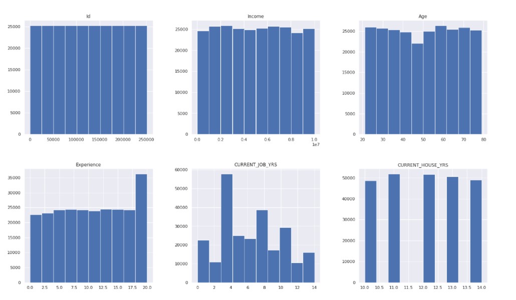
Now, we check the data distribution.
data.hist( figsize = (22, 20) )
plt.show()
Output:
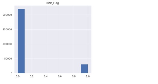
Now, we check the count of the target variable.
data["Risk_Flag"].value_counts()
Output:
0    221004
1     30996
Name: Risk_Flag, dtype: int64
Only a small part of the target variable consists of people who default on loans.
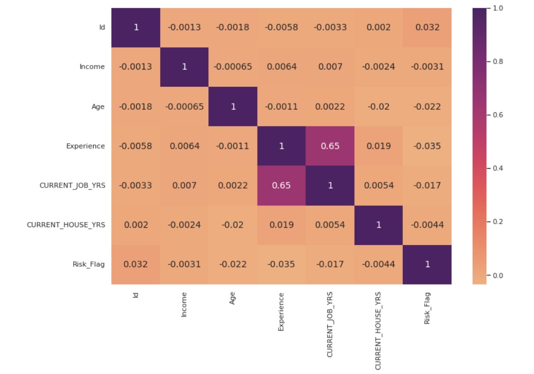
Now, we plot the correlation plot.
fig, ax = plt.subplots( figsize = (12,8) )
corr_matrix = data.corr()
corr_heatmap = sns.heatmap( corr_matrix, cmap = "flare", annot=True, ax=ax, annot_kws={"size": 14})
plt.show()
Output:
Analyzing Categorical Features
Now, we proceed with the analysis of categorical features.
First, we define a function to create the plots.
def categorical_valcount_hist(feature):
    print(data[feature].value_counts())
    fig, ax = plt.subplots( figsize = (6,6) )
    sns.countplot(x=feature, ax=ax, data=data)
    plt.show()
First, we check the count of married people vs single people.
categorical_valcount_hist("Married/Single")
Output:
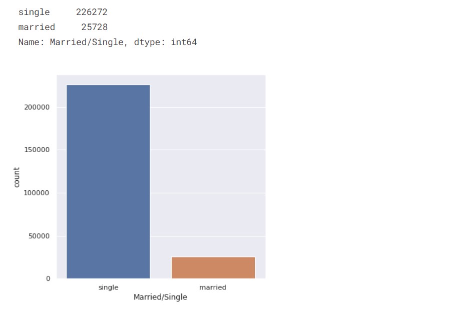
So, the majority of the people are single.
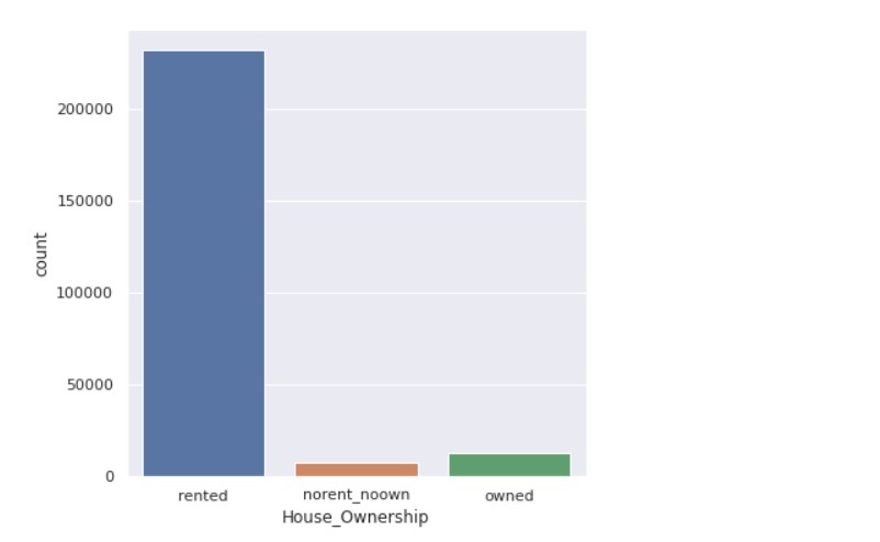
Now, we check the count of house ownership.
categorical_valcount_hist("House_Ownership")
Output:
Now, let us check the count of states.
print( "Total categories in STATE:", len( data["STATE"].unique() ) )
print()
print( data["STATE"].value_counts() )
Output:
Total categories in STATE: 29
Uttar_Pradesh        28400
Maharashtra          25562
Andhra_Pradesh       25297
West_Bengal          23483
Bihar                19780
Tamil_Nadu           16537
Madhya_Pradesh       14122
Karnataka            11855
Gujarat              11408
Rajasthan             9174
Jharkhand             8965
Haryana               7890
Telangana             7524
Assam                 7062
Kerala                5805
Delhi                 5490
Punjab                4720
Odisha                4658
Chhattisgarh          3834
Uttarakhand           1874
Jammu_and_Kashmir     1780
Puducherry            1433
Mizoram                849
Manipur                849
Himachal_Pradesh       833
Tripura                809
Uttar_Pradesh[5]       743
Chandigarh             656
Sikkim                 608
Name: STATE
dtype: int64
Now, we check the count of professions.
print( "Total categories in Profession:", len( data["Profession"].unique() ) )
print()
data["Profession"].value_counts()
Output:
Total categories in Profession: 51
Physician                     5957
Statistician                  5806
Web_designer                  5397
Psychologist                  5390
Computer_hardware_engineer    5372
Drafter                       5359
Magistrate                    5357
Fashion_Designer              5304
Air_traffic_controller        5281
Comedian                      5259
Industrial_Engineer           5250
Mechanical_engineer           5217
Chemical_engineer             5205
Technical_writer              5195
Hotel_Manager                 5178
Financial_Analyst             5167
Graphic_Designer              5166
Flight_attendant              5128
Biomedical_Engineer           5127
Secretary                     5061
Software_Developer            5053
Petroleum_Engineer            5041
Police_officer                5035
Computer_operator             4990
Politician                    4944
Microbiologist                4881
Technician                    4864
Artist                        4861
Lawyer                        4818
Consultant                    4808
Dentist                       4782
Scientist                     4781
Surgeon                       4772
Aviator                       4758
Technology_specialist         4737
Design_Engineer               4729
Surveyor                      4714
Geologist                     4672
Analyst                       4668
Army_officer                  4661
Architect                     4657
Chef                          4635
Librarian                     4628
Civil_engineer                4616
Designer                      4598
Economist                     4573
Firefighter                   4507
Chartered_Accountant          4493
Civil_servant                 4413
Official                      4087
Engineer                      4048
Name: Profession
dtype: int64
Data Analysis
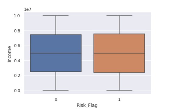
Now, we start with understanding the relationship between the different data features.
sns.boxplot(x ="Risk_Flag",y="Income" ,data = data)
Output:
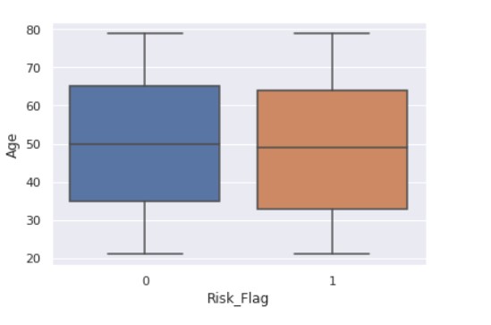
Now, we see the relationship between the flag variable and age.
sns.boxplot(x ="Risk_Flag",y="Age" ,data = data)
Output:
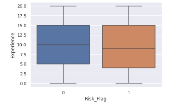
sns.boxplot(x ="Risk_Flag",y="Experience" ,data = data)
Output:
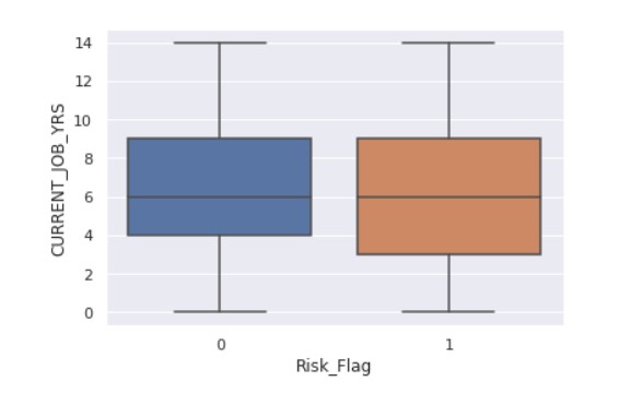
sns.boxplot(x ="Risk_Flag",y="CURRENT_JOB_YRS" ,data = data)
Output:
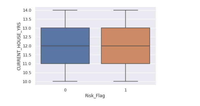
sns.boxplot(x ="Risk_Flag",y="CURRENT_HOUSE_YRS" ,data = data)
Output:
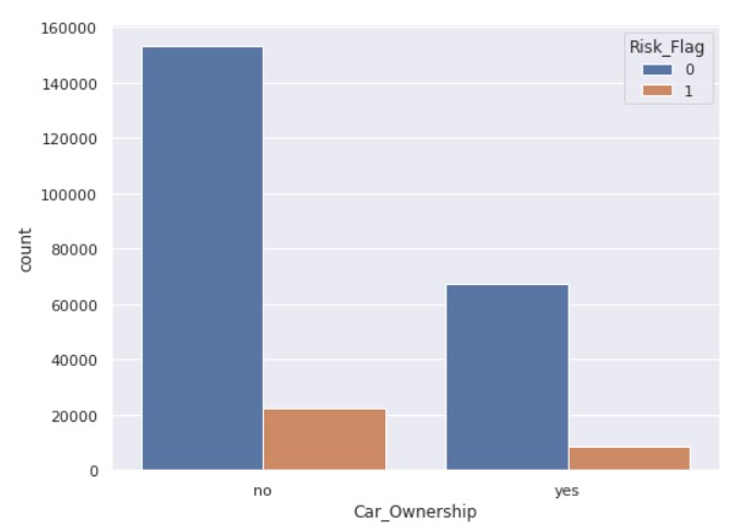
fig, ax = plt.subplots( figsize = (8,6) )
sns.countplot(x='Car_Ownership', hue='Risk_Flag', ax=ax, data=data)
Output:
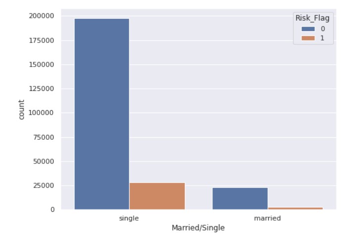
fig, ax = plt.subplots( figsize = (8,6) )
sns.countplot( x='Married/Single', hue='Risk_Flag', data=data )
Output:
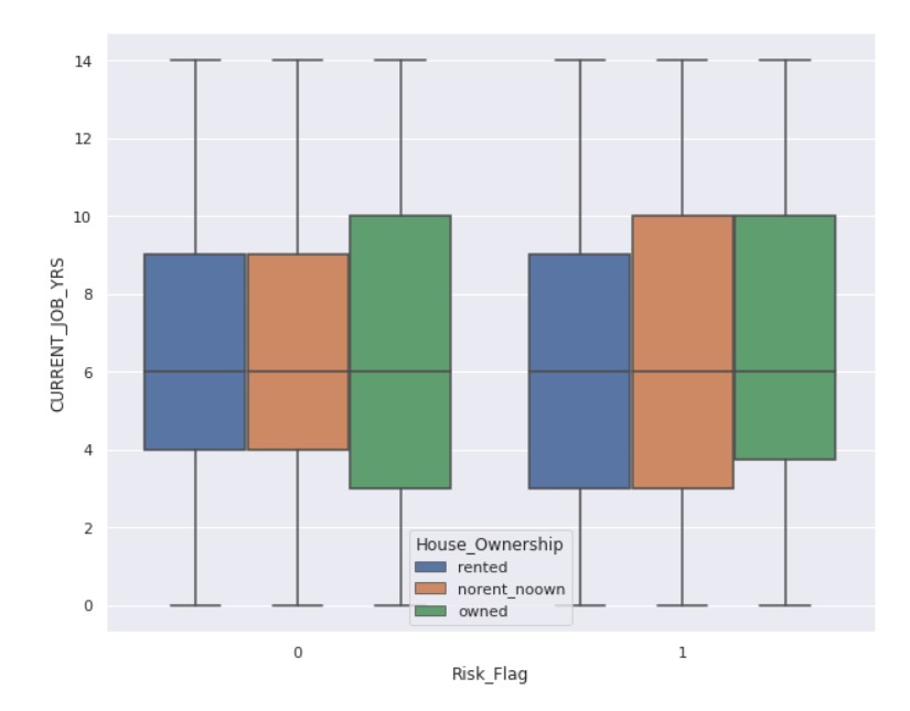
fig, ax = plt.subplots( figsize = (10,8) )
sns.boxplot(x = "Risk_Flag", y = "CURRENT_JOB_YRS", hue='House_Ownership', data = data)
Output:
Encoding
Data preparation is a required process in the field of data science before moving on to modelling. In the data preparation process, we must complete a number of tasks. One of these critical responsibilities is the encoding of categorical data. As we all know, most data in real life has categorical string values, and most machine learning models only deal with integer values or other values that can be understood by the model. All models, in essence, execute mathematical operations that may be carried out using a variety of tools and methodologies.
Encoding categorical data is the process of turning categorical data into integer format so that data with transformed categorical values may be fed into models to increase prediction accuracy.
We will apply encoding to the categorical features.
from sklearn.preprocessing import LabelEncoder
from sklearn.preprocessing import OneHotEncoder
import category_encoders as ce
label_encoder = LabelEncoder() for col in ['Married/Single','Car_Ownership']: data[col] = label_encoder.fit_transform( data[col] )
onehot_encoder = OneHotEncoder(sparse = False)
data['House_Ownership'] = onehot_encoder.fit_transform(data['House_Ownership'].values.reshape(-1, 1) )
high_card_features = ['Profession', 'CITY', 'STATE']
count_encoder = ce.CountEncoder()
# Transform the features, rename the columns with the _count suffix, and join to dataframe
count_encoded = count_encoder.fit_transform( data[high_card_features] )
data = data.join(count_encoded.add_suffix("_count"))
data= data.drop(labels=['Profession', 'CITY', 'STATE'], axis=1)
After the feature engineering part is complete, we shall split the data into training and testing sets.
Splitting the data into train and test splits
The train-test split is used to measure the performance of machine learning models relevant to prediction-based Algorithms/Applications. This approach is a quick and simple procedure that allows us to compare our own machine learning model outcomes to machine results. By default, the Test set is made up of 30% of the real data, whereas the Training set is made up of 70% of the actual data.
To assess how effectively our machine learning model works, we must divide a dataset into training and testing sets. The train set is used to train the Machine Learning model, and its statistics are known. The second set is known as the test data set, and it is only utilized for predictions.
It is an important part of the ML chain.
x = data.drop("Risk_Flag", axis=1)
y = data["Risk_Flag"]
from sklearn.model_selection import train_test_split
x_train, x_test, y_train, y_test = train_test_split(x, y, test_size = 0.2, stratify = y, random_state = 7)
We have taken the test size to be 20% of the entire data.
Random Forest Classifier
Tree-based algorithms are widely utilized in machine learning to handle supervised learning challenges. These algorithms are adaptable and can tackle virtually any issue (classification or regression).
When generating predictions on training samples in the areas they belong to, tree-based algorithms often employ the mean for continuous data or the mode for categorical features. They also generate forecasts with great accuracy, stability, and interpretability.
Random forest is a common tree-based supervised learning technique. It is also the most adaptable and user-friendly.
The approach may be used to address classification and regression issues. Random forest typically combines hundreds of decision trees and then trains each decision tree on a different sample of the data.
The random forest’s final predictions are calculated by averaging the forecasts of each individual tree. The advantages of random forests are numerous. Individual decision trees have a tendency to overfit the training data, but the random forest can alleviate this problem by averaging the prediction results from several trees. This provides random forests with a better prediction accuracy than a single decision tree.
Now, we train the model and perform the predictions.
from sklearn.ensemble import RandomForestClassifier
from imblearn.over_sampling import SMOTE
from imblearn.pipeline import Pipeline
rf_clf = RandomForestClassifier(criterion='gini', bootstrap=True, random_state=100)
smote_sampler = SMOTE(random_state=9)
pipeline = Pipeline(steps = [['smote', smote_sampler],
                             ['classifier', rf_clf]])
pipeline.fit(x_train, y_train)
y_pred = pipeline.predict(x_test)
Now, we check the accuracy scores.
from sklearn.metrics import confusion_matrix, precision_score, recall_score, f1_score, accuracy_score, roc_auc_score
print("-------------------------TEST SCORES-----------------------")
print(f"Recall: { round(recall_score(y_test, y_pred)*100, 4) }")
print(f"Precision: { round(precision_score(y_test, y_pred)*100, 4) }")
print(f"F1-Score: { round(f1_score(y_test, y_pred)*100, 4) }")
print(f"Accuracy score: { round(accuracy_score(y_test, y_pred)*100, 4) }")
print(f"AUC Score: { round(roc_auc_score(y_test, y_pred)*100, 4) }")
Output:
-------------------------TEST SCORES-----------------------
Recall: 54.1378
Precision: 54.3306
F1-Score: 54.234
Accuracy score: 88.7619
AUC Score: 73.8778
The accuracy scores might not be up to the mark, but this is the overall process of predicting loan default.
Code: Here
Conclusion
- The Random Forest approach is appropriate for classification and regression tasks on datasets with many entries and features that are likely to have missing values when we need a highly accurate result while avoiding overfitting.
- Furthermore, the random forest provides relative feature significance, enabling you to select the most important features. It is more interpretable than neural network models but less interpretable than decision trees.
- In the case of categorical features, we need to perform encoding so that the ML algorithm can process them.
- Predicting Loan Default is highly dependent on the demographics of the people, people with lower income are more likely to default on loans.
We are able to successfully perform the classification task using Random Forest Classifier. Hope you liked my article on predicting loan default.
The media shown in this article is not owned by Analytics Vidhya and are used at the Author’s discretion.


