This article was published as a part of the Data Science Blogathon.
Introduction
In this article, I will explain linear Regression, one of the machine learning algorithms. After reading this, we will get some basic knowledge about linear Regression, its uses, its types, and so on. Let us start with the table of contents.
Table of contents
What is Linear Regression
Uses of Linear Regression
Selection Criteria
When will Linear Regression be used?
Types of Linear Regression
Understanding Linear Regression
How to find the effectiveness of the model?
R Square method
Regression analysis is a form of predictive modeling technique that investigates the relationship between X and Y, where x is the independent variable Y is the dependent variable.
Types of Regression – There are two types of Regression. One is linear Regression used with continuous variables, and the other is logistic Regression used with categorical variables.
Linear Regression
Regression analysis is graphing a line on a set of data points that most closely fits the overall shape of the data.
In other words, Regression shows the changes in a dependent variable on the y-axis to the changes in the explanatory variable on the x-axis.
Uses of Regression
- We determine the strength of predictors, for example, the relation between sales and marketing spending or the connection between age and income.
- It is forecasting an effect and is used to predict the impact or impact of changes. This is used to understand how much the dependent variable changes with the evolution of the independent variable. For example, how much sales are increased with extra 1000 rupees spent on marketing?
- Trend forecasting. This can be used to get the point estimates.
Selection Criteria
- Classification and regression capabilities: Predicts the continuous variable (For example-Temperature of a place)
- Data quality: Each missing point removes one data point that could optimize the Regression.
- Computational complexity: Linear Regression is not always computationally expensive than the decision tree or the clustering algorithm.
- Comprehensible and Transparent: Linear Regression is easily understandable, and a simple mathematical notation can represent transparency.
Where will Linear Regression be used?
- Evaluating trends and sales estimates
- Analyzing the impact of price changes
- Estimation of risk in financial services and insurance domain
Types of Linear Regression
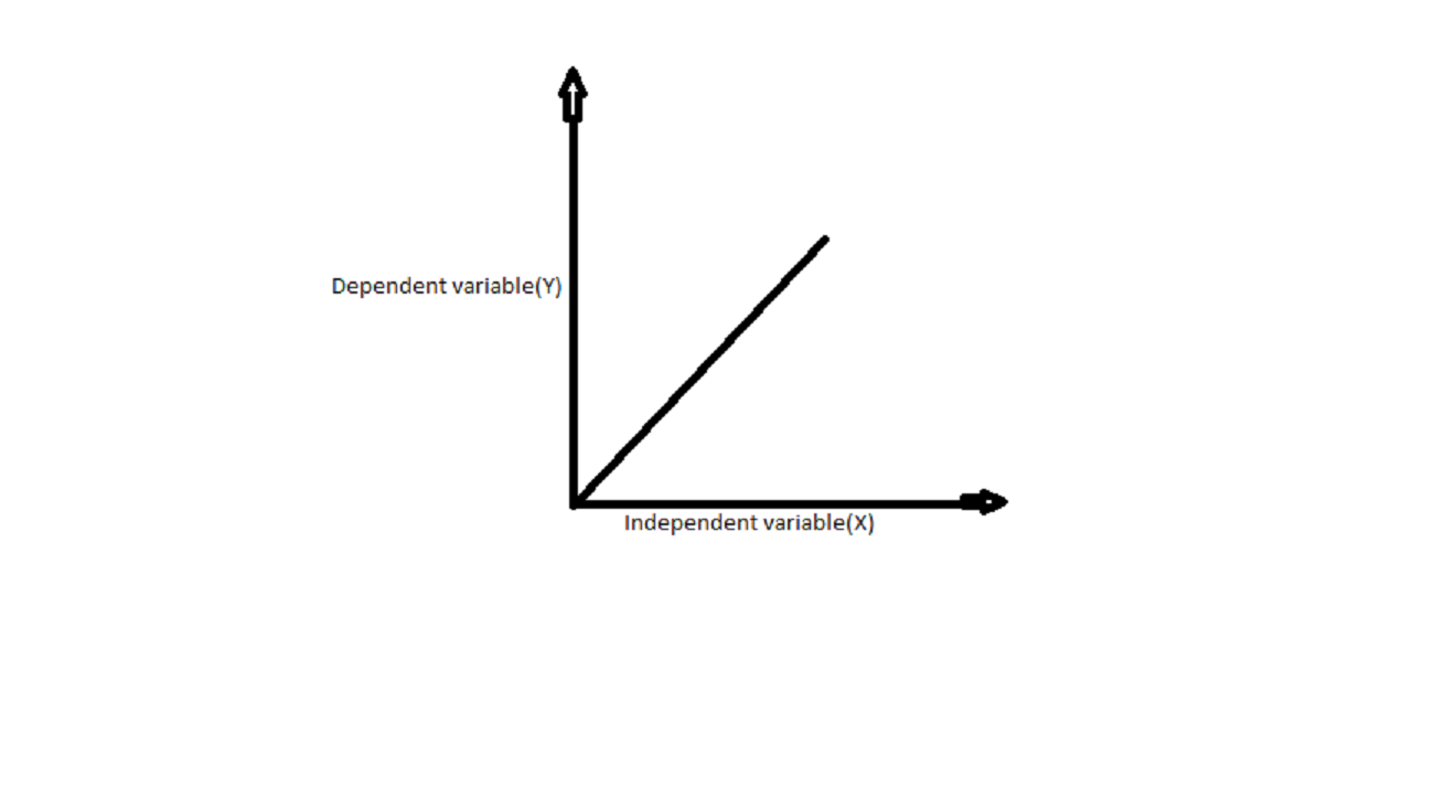
Linear Regression is of two types. One is positive Linear Regression, and the other is negative Linear Regression.
Positive Linear Regression– If the value of the dependent variable increases with the increase of the independent variable, then the slope of the graph is positive; such Regression is said to be Positive Linear Regression.

Source: Author
y=mx+c, where m is the slope of the line. In Positive Linear Regression, the value of m is positive.
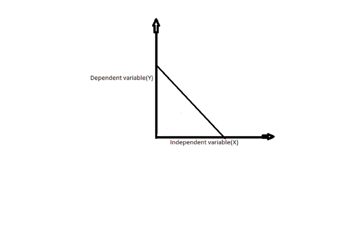
Negative Linear Regression- If the value of the dependent variable decreases with the increase in the value of the independent variable, then such Regression is said to be negative linear Regression.

Source: Author
In Negative Linear Regression, the value of m is Negative.
Understanding Linear Regression
First of all, we need to have some data set to design the model.
Let us say the data is as below
| x | y |
| 1 | 3 |
| 2 | 4 |
| 3 | 2 |
| 4 | 4 |
| 5 | 5 |
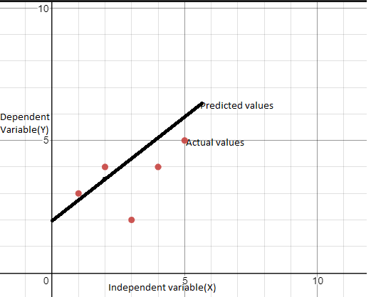
The values given are actual values.
Based on the above matters, the graph that most closely fits is as below
y=mx+c, where m is the slope of the line and c is Y-intercept.
From now on x(mean) is referred as x(m) and y(mean) as y(m).
m as per least square method=∑(x-x(m))(y-y(m))/∑(x-x(m))2
As per above data table, x(m)=3, y(m)=3.6.
| x | y | x-x(m) | y-y(m) | (x-x(m))2 | (y-y(m))2 |
| 1 | 3 | -2 | -0.6 | 4 | 1.2 |
| 2 | 4 | -1 | 0.4 | 1 | -0.4 |
| 3 | 2 | 0 | -1.6 | 0 | 0 |
| 4 | 4 | 1 | 0.4 | 1 | 0.4 |
| 5 | 5 | 2 | 1.4 | 4 | 2.8 |
As per the equation of m, its value is m=4/10=0.4,c=2.4, so that the line equation would be y=0.4x+2.4.
x-x(m) is the distance of all the points x through the line y=3.
y-y(m) is the distance of all the points y through the line x=3.6.
Now we will calculate the predicted values of y based on the equation y=mx+c, where m=0.4 and c=2.4.
For x=1,y=0.4*1+2.4=2.8
For x=2,y=0.4*2+2.4=3.2
For x=3,y=0.4*3+2.4=3.6
For x=4,y=0.4*4+2.4=4.0
For x=5,y=0.4*5+2.4=4.4
Now we have actual values and predicted values of y; we need to calculate the distance between them and then reduce them, which means we need to reduce the error, and finally, the line with the minor error would be the line of Regression best fit line.
Finding the best fit line:
For different values of m, we need to calculate the line equation, where y=mx+c as the value of m changes, the equation changes. After every iteration, the predicted value changes according to the line’s equation. It needs to compare with the actual value and the importance of m for which the minimum difference gives the best fit line.
Let’s check the goodness of fit:
To test how good our model is performing, we have a method called the R Square method
R square method
This method is based on a value called the R-Squared value. It measures how close the data is to the regression line—and also known as the coefficient of determination.

Source: Author
To check our model’s good, we need to compare the distance between the actual value and mean versus the distance between the predicted value and mean; here comes the R formula.
R2=∑(yp-y(m))2/∑(y-y(m))2
If the value of R2 is nearer to 1, then the model is more effective
If the value of R2 is far away from 1, then the model is least effective
| x | y | y-y(m) | (y-y(m))2 | yp | (yp-y(m))2 |
| 1 | 3 | -0.6 | 0.36 | 2.8 | -0.8 |
| 2 | 4 | 0.4 | 0.16 | 3.2 | -0.4 |
| 3 | 2 | -1.6 | 2.56 | 3.6 | 0 |
| 4 | 4 | 0.4 | 0.16 | 4.0 | 0.4 |
| 5 | 5 | 1.4 | 1.96 | 4.4 | 0.8 |
R2=1.6/5.2=0.3
This means that the data points are far away from the regression line.
If the value of R is 1, then the actual data points would be on the regression line.
Conclusion
We have covered all the topics related to Linear Regression. And we also found the effectiveness of the model using the R square method. For example, R-value might come close to 1 if the data is regarding a company’s sales. R-value might be too low if the information is from a doctor in psychology since different persons have different characters. So the conclusion is if the R-value is closer to one, the more accurate is the predicted value.
Thanks for reading this article. Learn more here.
Connect with me on https://www.instagram.com/?hl=en.
Image Source: Author.
The media shown in this article is not owned by Analytics Vidhya and are used at the Author’s discretion.


