Building an End-to-End Logistic Regression Model

Logistic regression is a statistical model used to analyze and predict binary outcomes. It’s commonly used in finance, marketing, healthcare, and social sciences to model and predict binary outcomes. A logistic regression model uses a logistic function to model the probability of a binary response variable, given one or more predictor variables. In this article, we will be discussing the logistic regression model in detail.

This article was published as a part of the Data Science Blogathon

What is Machine Learning?

Machine Learning algorithms can access data (categorical, numerical, image, video, or anything) and use it to learn for themselves without any explicit programming. But how does the Machine Learning technique work? just by observing the data (through instructions to observe the pattern and making decisions or predictions)

Types of Machine Learning

Machine Learning algorithmic techniques can be broadly classified into three types,

• Supervised Machine Learning – Task Driven (Classification and Regression)
• Unsupervised Machine Learning – Data-Driven (Clustering)
• Reinforcement Machine Learning – Learning from mistakes (Rewards or Punishment)

Supervised Machine Learning

Algorithms are trained in supervised learning utilizing labeled datasets, where the algorithm learns about each category of input. When the training phase is finished, the algorithm is evaluated on test data (a subset of the training set) and predicts the result. Supervised Machine Learning is classified into two types,

Regression

If there is a link between the input variable and the output variable, regression procedures are applied. It is used to forecast continuous variables such as weather, market trends, and so on.

Classification

When the output variable is categorical, such as Yes-No, Male-Female, True-False, Normal – Abnormal, and so on, classification methods are used.

What is Logistic Regression Model?

Logistic regression estimates the relationship between a dependent variable and one or more independent variables and predicts a categorical variable versus a continuous one. Here are a few things to know about logistic regression:

• Logistic regression is a Machine Learning method used for classification tasks.
• It is a predictive analytic technique based on the probability idea.
• The dependent variable in logistic regression is binary (coded as 1 or 0).
• The goal is to discover a link between characteristics and the likelihood of a specific outcome.
• Logistic regression uses a more sophisticated cost function called the “Sigmoid function” or “logistic function” instead of a linear function.
• The logistic regression hypothesis limits the cost function to a value between 0 and 1, making linear functions unsuitable for this task.
• Logistic regression is used in many fields, such as finance, marketing, healthcare, and social sciences, to model and predict binary outcomes.

Behind every great leader, there was an even greater logistician.

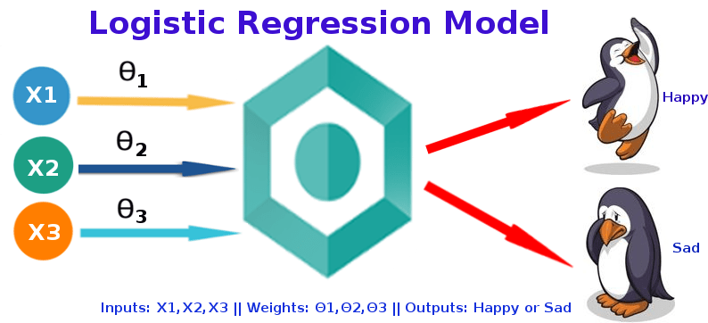
Logistic Regression is considered a regression model also. This model creates a regression model to predict the likelihood that a given data entry belongs to the category labeled “1.” Logistic regression models the data using the sigmoid function, much as linear regression assumes that the data follows a linear distribution.

Why the Name Logistic Regression?

It’s called ‘Logistic Regression’ since the technique behind it is quite similar to Linear Regression. The name “Logistic” comes from the Logit function, which is utilized in this categorization approach.

Why Can’t we use Linear Regression Instead of Logistic Regression?

Before answering this question, we will explain from Linear Regression concept, from the scratch then only we can understand it better. Although logistic regression is a sibling of linear regression, it is a classification technique, despite its name. Mathematically linear regression can be explained by,

• y = mx + c
• y – predicted value
• m – slope of the line
• x – input data
• c- Y-intercept or slope

We can forecast y values such as using these values. Now observe the below diagram for a better understanding,

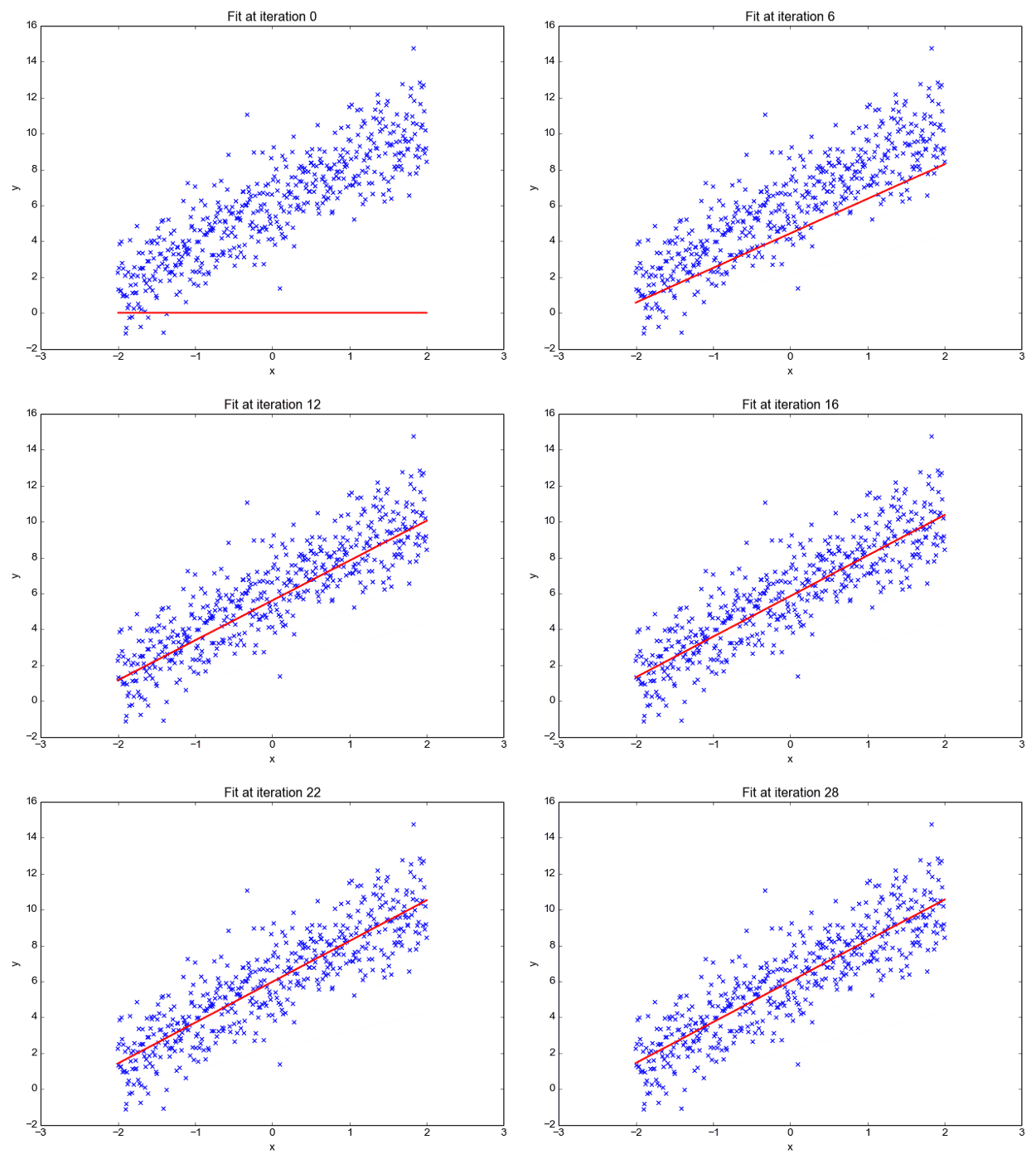
The x values are represented by the blue dots (the input data). We can now compute slope and y coordinate using the input data to ensure that our projected line (red line) covers most of the locations. We can now forecast any value of y given its x values using this line.

One thing to keep in mind about linear regression is that it only works with continuous data. If we want to include linear regression in our classification methods, we’ll have to adjust our algorithm a little more. First, we must choose a threshold so that if our projected value is less than the threshold, it belongs to class 1; otherwise, it belongs to class 2.

Now, if you’re thinking, “Oh, that’s simple, just create linear regression with a threshold, and hurray!, classification method,” there’s a catch. We must specify the threshold value manually, and calculating the threshold for huge datasets will be impossible. Furthermore, even if our anticipated values vary, the threshold value will remain the same. A logistic regression, on the other hand, yields a logistic curve with values confined to 0 and 1. The curve in logistic regression is generated using the natural logarithm of the target variable’s “odds,” rather than the probability, as in linear regression. Furthermore, the predictors need not be regularly distributed or have the same variance in each group.

And Now the Question?

This famous title question was explained by our beloved person Andrew Ng, assume we have information about tumor size and malignancy. Because this is a classification issue, we can see that all the values will fall between 0 and 1. And, by fitting the best-found regression line and assuming a threshold of 0.5, we can do a very good job with the line.

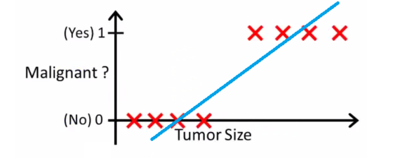
We can choose a point on the x-axis from which all values on the left side are regarded as negative, and all values on the right side are considered positive.

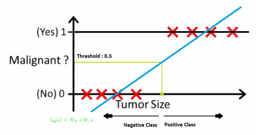
But what if the data contains an outlier? Things would become shambles. For 0.5 thresholds, for example,

Even if we fit the best-found regression line, we won’t be able to determine any point where we can distinguish classes. It will insert some instances from the positive class into the negative class. The green dotted line (Decision Boundary) separates malignant and benign tumors, however, it should have been a yellow line that clearly separates the positive and negative cases. As a result, even a single outlier can throw the linear regression estimates off. And it’s here that logistic regression comes into play.

Logit function to Sigmoid Function

Logistic Regression can be expressed as,

where p(x)/(1-p(x)) is termed odds, and the left-hand side is called the logit or log-odds function. The odds are the ratio of the chances of success to the chances of failure. As a result, in Logistic Regression, a linear combination of inputs is translated to log(odds), with an output of 1.

The following is the inverse of the aforementioned function

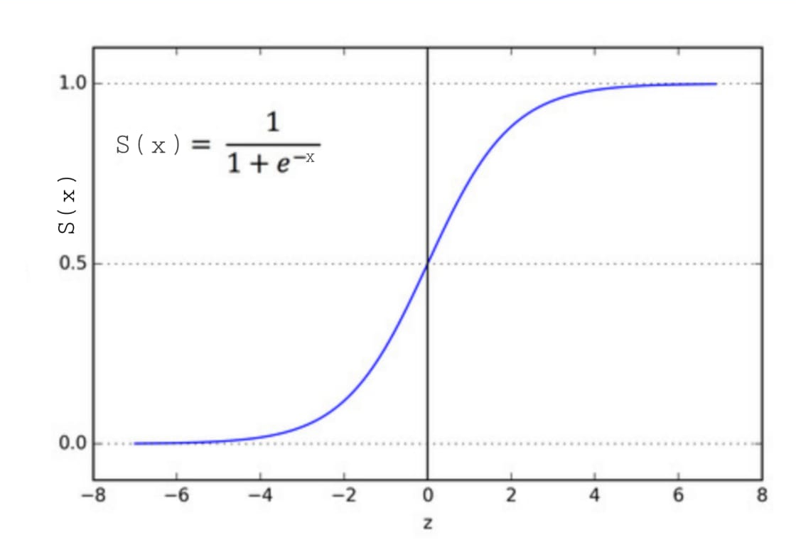
This is the Sigmoid function, which produces an S-shaped curve. It always returns a probability value between 0 and 1. The Sigmoid function is used to convert expected values to probabilities. The function converts any real number into a number between 0 and 1. We utilize sigmoid to translate predictions to probabilities in machine learning.

The mathematically sigmoid function can be,

Types of Logistic Regression

In general, it can be classified into,

1. Binary Logistic Regression – two or binary outcomes like yes or no
2. Multinomial Logistic Regression – three or more outcomes like first, second, and third class or no class degree
3. Ordinal Logistic Regression – three or more like multinomial logistic regression but here with the order like customer rating in the supermarket from 1 to 5

Requirements for Logistic Regression

This model can work for all the datasets, but still, if you need good performance, then there will be some assumptions to consider,

• The dependant variable in binary logistic regression must be binary.
• Only the variables that are relevant should be included.
• The independent variables must be unrelated to one another. That is, there should be minimal or no multicollinearity in the model.
• The log chances are proportional to the independent variables.
• Large sample sizes are required for logistic regression.

Decision Boundary – Logistic Regression

A threshold can be established to forecast which class a data belongs to. The derived estimated probability is categorized into classes based on this threshold.

If the predicted value is less than 0.5, categorize the particular student as a pass; otherwise, label it as a fail. There are two types of decision boundaries: linear and non-linear. To provide a complicated decision boundary, the polynomial order can be raised.

Why can’t the cost function that was used for linearity be used for logistics?

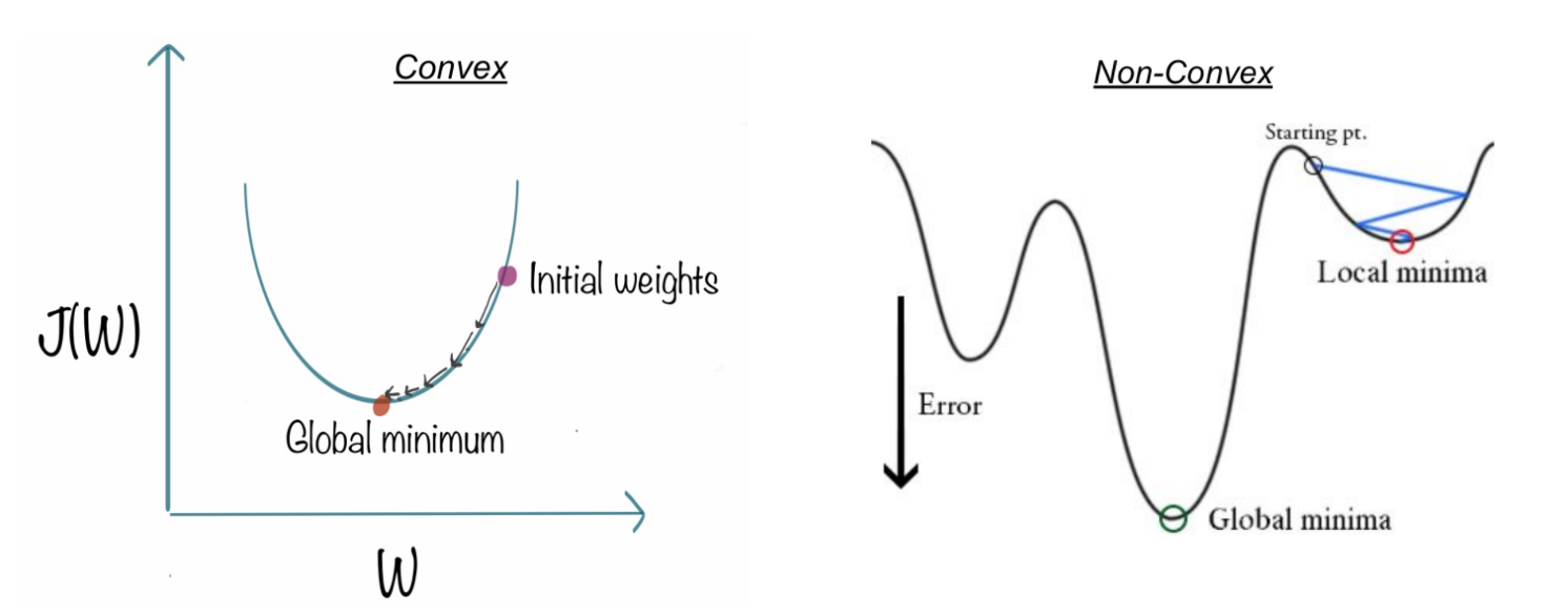
The cost function for linear regression is mean squared error. If this is utilized for logistic regression, the function of parameters will be non-convex. Only if the function is convex will gradient descent lead to a global minimum.

Cost function – Linear Regression Vs Logistic Regression

Linear regression employs the Least Squared Error as the loss function, which results in a convex network, which we can then optimize by identifying the vertex as the global minimum. For logistic regression, however, it is no longer a possibility. Because the hypothesis has been modified, calculating Least Squared Error using the sigmoid function on raw model output will result in a non-convex graph with local minimums.

What is cost function? Cost functions are used in machine learning to estimate how poorly models perform. Simply put, a cost function is a measure of how inaccurate the model is in estimating the connection between X and y. This is usually stated as a difference or separation between the expected and actual values. A machine learning model’s goal is to discover parameters, weights, or a structure that minimizes the cost function.

A convex function indicates there will be no intersection between any two points on the curve, but a non-convex function will have at least one intersection. In terms of cost functions, a convex type always guarantees a global minimum, whereas a non-convex type only guarantees local minima.

How to Reduce Cost Function? – Gradient Descent

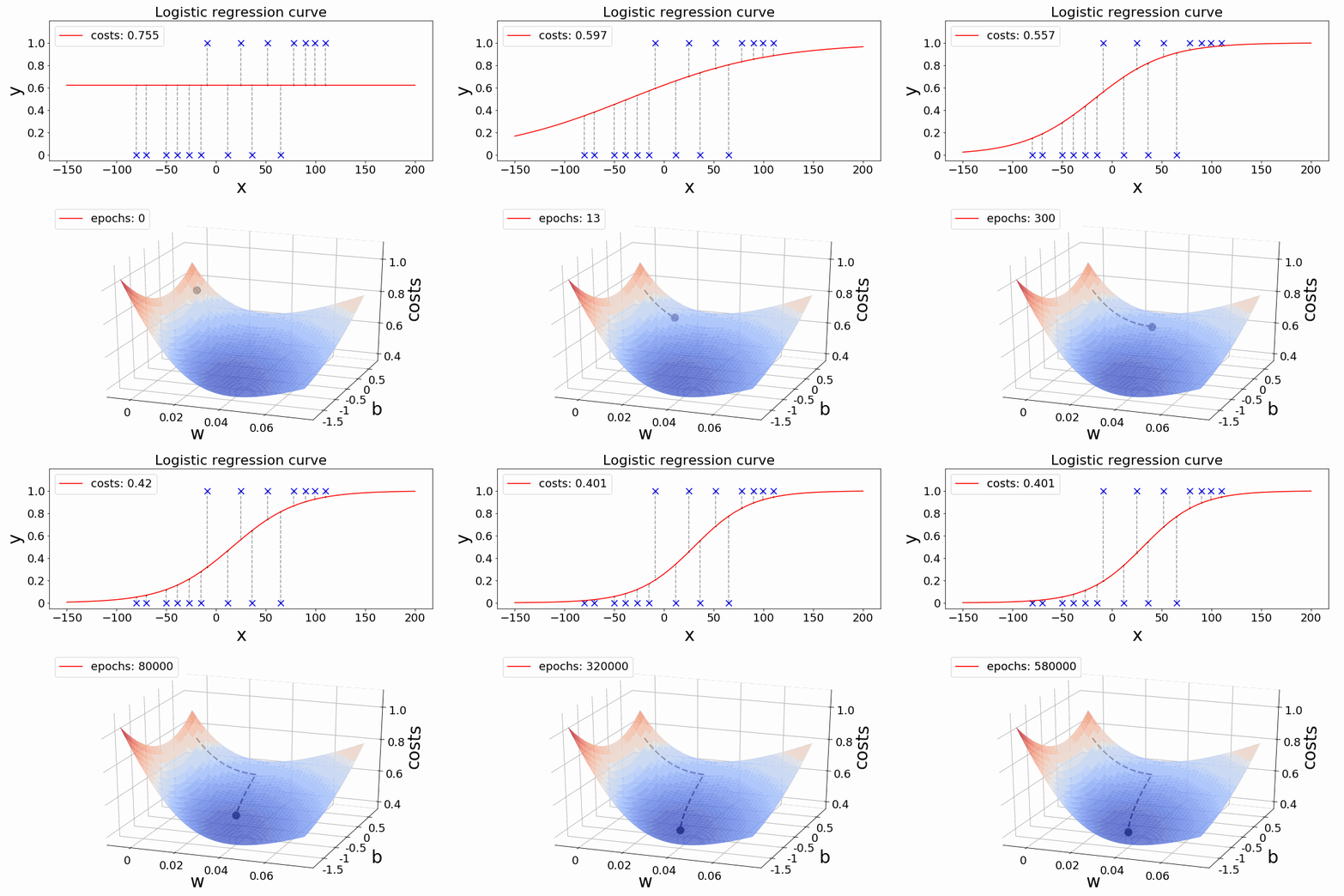
The challenge now is: how can we lower the cost value? Gradient Descent can be used to accomplish this. Gradient descent’s main objective is to reduce the cost value.

Regularization

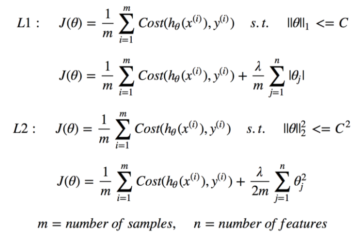
Let’s also discuss Regularization quickly for reducing the cost function to match the parameters to training data. L1 (Lasso) and L2 (Lasso) are the two most frequent regularization types (Ridge). Instead of simply maximizing the aforementioned cost function, regularization imposes a limit on the size of the coefficients in order to avoid overfitting. L1 and L2 use distinct approaches to defining upper limits for coefficients, allowing L1 to conduct feature selection by setting coefficients to 0 for less relevant characteristics and reducing multi-collinearity, whereas L2 penalizes extremely large coefficients but does not set any to 0. There’s also a parameter that regulates the constraint’s weight, λ, to ensure that coefficients aren’t penalized too harshly, resulting in underfitting.

It’s a fascinating topic to investigate why L1 and L2 have different capacities owing to the ‘squared’ and ‘absolute’ values, and how λ affects the weight of regularized and original fit terms. We won’t go into everything here, but it’s well worth your time and effort to learn about. The steps below demonstrate how to convert an original cost function to a regularized cost function.

How Logistic Regression links with Neural Network?

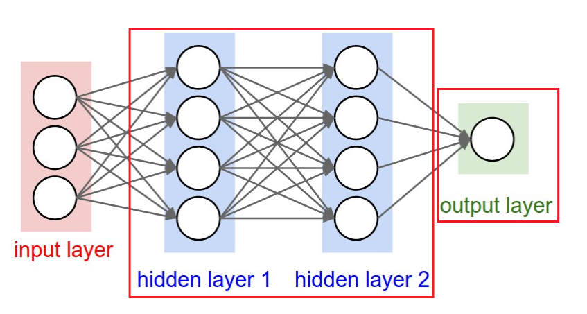
We all know that Neural Networks are the foundation for Deep Learning. The best part is that Logistic Regression is intimately linked to Neural networks. Each neuron in the network may be thought of as a Logistic Regression; it contains input, weights, and bias, and you conduct a dot product on all of that before applying any non-linear function. Furthermore, a neural network’s last layer is a basic linear model (most of the time). That can be understood by visualization as shown below,

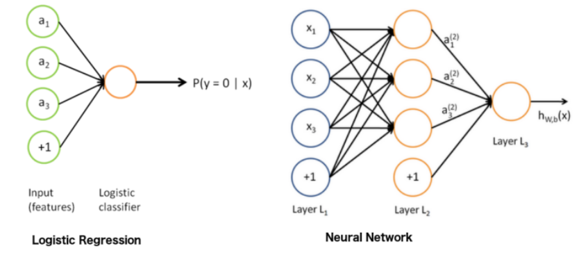
Take a deeper look at the “output layer,” and you’ll notice that it’s a basic linear (or logistic) regression: we have the input (hidden layer 2), the weights, a dot product, and finally a non-linear function, depends on the task. A helpful approach to thinking about neural networks is to divide them into two parts: representation and classification/regression. The first section (on the left) aims to develop a decent data representation that will aid the second section (on the right) is doing a linear classification/regression.

 Hyperparameter Fine-tuning – Logistic Regression

There are no essential hyperparameters to adjust in logistic regression. Even though it has many parameters, the following three parameters might be helpful in fine-tuning for some better results,

Regularization (penalty) might be beneficial at times.

Penalty – {‘l1’, ‘l2’, ‘elasticnet’, ‘none’}, default=’l2’

The penalty strength is controlled by the C parameter, which might be useful.

C – float, default=1.0

With different solvers, you might sometimes observe useful variations in performance or convergence.

Solver – {‘newton-cg’, ‘lbfgs’, ‘liblinear’, ‘sag’, ‘saga’}, default=’lbfgs’

Note: The algorithm to use is determined by the penalty: Solver-supported penalties:

• ‘newton-cg’ – [‘l2’, ‘none’]
• ‘lbfgs’ – [‘l2’, ‘none’]
• ‘liblinear’ – [‘l1’, ‘l2’]
• ‘sag’ – [‘l2’, ‘none’]
• ‘saga’ – [‘elasticnet’, ‘l1’, ‘l2’, ‘none’]

Python Implementation

Dataset: https://www.kaggle.com/uciml/breast-cancer-wisconsin-data 

Whenever we start writing the program, always our first step is to start with importing libraries,

Next to importing libraries, it’s our data to import, either from local disk or from url link

Before getting into modeling, we need to understand the statistical importance for better understanding,

dataset.info()

dataset.shape

dataset.describe().T

print(str('Any missing data or NaN in the dataset:'),dataset.isnull().values.any())

If you understand the correlation between the features, it will be easy to process, like adding for modeling or removing

corr_var=dataset.corr()
print(corr_var)
plt.figure(figsize=(10,7.5))
sns.heatmap(corr_var, annot=True, cmap='BuPu')

X = dataset.iloc[:,:-1].values
y = dataset.iloc[:,-1].values

from sklearn.model_selection import train_test_split
X_train, X_test, y_train, y_test = train_test_split (X, y, test_size=0.2, random_state=0)
print('Total no. of samples: Training and Testing dataset separately!')
print('X_train:', np.shape(X_train))
print('y_train:', np.shape(y_train))
print('X_test:', np.shape(X_test))
print('y_test:', np.shape(y_test))

from sklearn.preprocessing import StandardScaler
sc = StandardScaler()
X_train = sc.fit_transform(X_train)
X_test = sc.transform(X_test)

from sklearn.linear_model import LogisticRegression
classifier7 = LogisticRegression()
classifier7.fit(X_train,y_train)

y_pred7 = classifier7.predict(X_test)
print(np.concatenate((y_pred7.reshape(len(y_pred7),1), y_test.reshape(len(y_test),1)),1))

from sklearn.metrics import confusion_matrix, accuracy_score, roc_auc_score
cm7 = confusion_matrix(y_test, y_pred7)
print(cm7)

from mlxtend.plotting import plot_confusion_matrix
fig, ax = plot_confusion_matrix(conf_mat=cm7, figsize=(6, 6), cmap=plt.cm.Greens)
plt.xlabel('Predictions', fontsize=18)
plt.ylabel('Actuals', fontsize=18)
plt.title('Confusion Matrix', fontsize=18)
plt.show()

logreg=accuracy_score(y_test,y_pred7)
logreg

Then finally, AUC-ROC score value, closer to 1 makes the system more accurate

roc_auc_score(y_test, y_pred7)

Overall metrics report of the logistic regression by Precision, Recall, F1 Score makes more understanding by how detailed our model predicts the data

import sklearn.metrics as metrics
print(metrics.classification_report(y_test, y_pred7))

Hyperparameter makes our model more fine-tune the parameters and also we can manually fine-tune our parameters for robust model and can see the difference in importance of using parameters

from sklearn.model_selection import GridSearchCV
parameters_lr = [{'penalty':['l1','l2'],'C': [0.001, 0.01, 0.1, 1, 10, 100, 1000]}]
grid_search_lr = GridSearchCV(estimator = classifier7,
                           param_grid = parameters_lr,
                           scoring = 'accuracy',
                           cv = 10,
                           n_jobs = -1)
grid_search_lr.fit(X_train, y_train)
best_accuracy_lr = grid_search_lr.best_score_
best_paramaeter_lr = grid_search_lr.best_params_  
print("Best Accuracy of LR: {:.2f} %".format(best_accuracy_lr.mean()*100))
print("Best Parameter of LR:", best_paramaeter_lr)

Advantages of Logistic Regression

1. Overfitting is less likely with logistic regression, although it can happen in high-dimensional datasets. In these circumstances, regularization (L1 and L2) techniques may be used to minimize over-fitting.
2. It works well when the dataset is linearly separable and has good accuracy for many basic data sets.
3. It is more straightforward to apply, understand, and train.
4. The inferences regarding the relevance of each characteristic are based on the anticipated parameters (trained weights). The association’s orientation, positive or negative, is also specified. As a result, logistic regression may be used to determine the connection between the characteristics.
5. Unlike decision trees or support vector machines, this technique allows models to be readily changed to incorporate new data. Stochastic gradient descent can be used to update the data.
6. It is less prone to over-fitting in a low-dimensional dataset with enough training instances.
7. When the dataset includes linearly separable characteristics, Logistic Regression shows to be highly efficient.
8. It has a strong resemblance to neural networks. A neural network representation may be thought of as a collection of small logistic regression classifiers stacked together.
9. The training time of the logistic regression method is considerably smaller than that of most sophisticated algorithms, such as an Artificial Neural Network, due to its simple probabilistic interpretation.
10. Multinomial Logistic Regression is the name given to an approach that may easily be expanded to multi-class classification using a softmax classifier.

Disadvantages of Logistic Regression

1. Logistic Regression should not be used if the number of observations is fewer than the number of features; otherwise, it may result in overfitting.
2. Because it creates linear boundaries, we won’t obtain better results when dealing with complex or non-linear data.
3. It’s only good for predicting discrete functions. As a result, the Logistic Regression dependent variable is restricted to the discrete number set.
4. The average or no multicollinearity between independent variables is required for logistic regression.
5. Logistic regression needs a big dataset and enough training samples to identify all of the categories.
6. Because this method is sensitive to outliers, the presence of data values in the dataset that differs from the anticipated range may cause erroneous results.
7. Only significant and relevant features should be utilized to construct a model; otherwise, the model’s probabilistic predictions may be inaccurate, and its predictive value may suffer.
8. Complex connections are difficult to represent with logistic regression. This technique is readily outperformed by more powerful and sophisticated algorithms such as Neural Networks.
9. Because logistic regression has a linear decision surface, it cannot address nonlinear issues. In real-world settings, linearly separable data is uncommon. As a result, non-linear features must be transformed, which may be done by increasing the number of features such that the data can be separated linearly in higher dimensions.
10. Based on independent variables, a statistical analysis model seeks to predict accurate probability outcomes. On high-dimensional datasets, this may cause the model to be over-fit on the training set, overstating the accuracy of predictions on the training set, and so preventing the model from accurately predicting outcomes on the test set. This is most common when the model is trained on a little amount of training data with many features. Regularization strategies should be explored on high-dimensional datasets to minimize over-fitting (but this makes the model complex). The model may be under-fit on the training data if the regularization parameters are too high.

Application of Logistic Regression

All use cases where data must be categorized into multiple groups are covered by Logistic Regression. Consider the following illustration:

1. Fraud detection in Credit card
2. Email spam or ham
3. Sentiment Analysis in Twitter analysis
4. Image segmentation, recognition, and classification – X-rays, Scans
5. Object detection through video
6. Handwriting recognition
7. Disease prediction – Diabetes, Cancer, Parkinson etc…

End Notes

The logistic Regression model is a powerful technique used for binary classification tasks. It is widely used in various fields, such as finance, marketing, healthcare, and social sciences, to model and predict binary outcomes. Our Blackbelt program is an excellent resource for individuals learning more about machine learning and advanced analytics. The program covers various topics, including data preparation, feature engineering, model selection, and evaluation techniques. Sign-up today!

The media shown in this article are not owned by Analytics Vidhya and are used at the Author’s discretion.

Premanand S

27 Apr 2023

Learner, Assistant Professor Junior & Machine Learning enthusiast