This article was published as a part of the Data Science Blogathon

Introduction
In this article, we will discuss the mathematical intuition behind Naive Bayes Classifiers, and we’ll also see how to implement this on Python.
This model is easy to build and is mostly used for large datasets. It is a probabilistic machine learning model that is used for classification problems. The core of the classifier depends on the Bayes theorem with an assumption of independence among predictors. That means changing the value of a feature doesn’t change the value of another feature.
Why is it called Naive?
It is called Naive because of the assumption that 2 variables are independent when they may not be. In a real-world scenario, there is hardly any situation where the features are independent.
Naive Bayes does seem to be a simple yet powerful algorithm. But why is it so popular?
Since it is a probabilistic approach, the predictions can be made real quick. It can be used for both binary and multi-class classification problems.
Before we dive deeper into this topic we need to understand what is “Conditional probability”, what is “Bayes’ theorem” and how conditional probability help’s us in Bayes’ theorem.
Table of contents
Conditional Probability for Naive Bayes
Conditional probability is defined as the likelihood of an event or outcome occurring, based on the occurrence of a previous event or outcome. Conditional probability is calculated by multiplying the probability of the preceding event by the updated probability of the succeeding, or conditional, event.
Let’s start understanding this definition with examples.
Suppose I ask you to pick a card from the deck and find the probability of getting a king given the card is clubs.
Observe carefully that here I have mentioned a condition that the card is clubs.
Now while calculating the probability my denominator will not be 52, instead, it will be 13 because the total number of cards in clubs is 13.
Since we have only one king in clubs the probability of getting a KING given the card is clubs will be 1/13 = 0.077.
Let’s take one more example,
Consider a random experiment of tossing 2 coins. The sample space here will be:
S = {HH, HT, TH, TT}
If a person is asked to find the probability of getting a tail his answer would be 3/4 = 0.75
Now suppose this same experiment is performed by another person but now we give him the condition that both the coins should have heads. This means if event A: ‘Both the coins should have heads’, has happened then the elementary outcomes {HT, TH, TT} could not have happened. Hence in this situation, the probability of getting heads on both the coins will be 1/4 = 0.25
From the above examples, we observe that the probability may change if some additional information is given to us. This is exactly the case while building any machine learning model, we need to find the output given some features.
Mathematically, the conditional probability of event A given event B has already happened is given by:
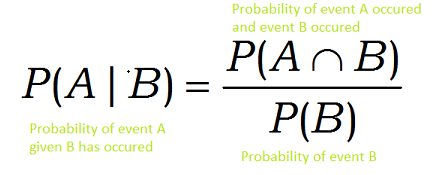
Image Source: Author
Bayes’ Rule
Now we are prepared to state one of the most useful results in conditional probability: Bayes’ Rule.
Bayes’ theorem which was given by Thomas Bayes, a British Mathematician, in 1763 provides a means for calculating the probability of an event given some information.
Mathematically Bayes’ theorem can be stated as:

Basically, we are trying to find the probability of event A, given event B is true.
Here P(B) is called prior probability which means it is the probability of an event before the evidence
P(B|A) is called the posterior probability i.e., Probability of an event after the evidence is seen.
With regards to our dataset, this formula can be re-written as:

Y: class of the variable
X: dependent feature vector (of size n)
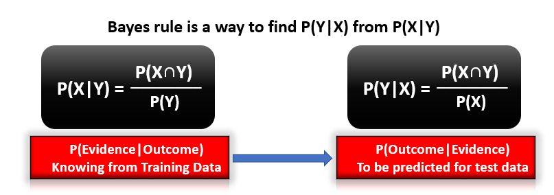
Image Source: Author
What is Naive Bayes?
Bayes’ rule provides us with the formula for the probability of Y given some feature X. In real-world problems, we hardly find any case where there is only one feature.
When the features are independent, we can extend Bayes’ rule to what is called Naive Bayes which assumes that the features are independent that means changing the value of one feature doesn’t influence the values of other variables and this is why we call this algorithm “NAIVE”
Naive Bayes can be used for various things like face recognition, weather prediction, Medical Diagnosis, News classification, Sentiment Analysis, and a lot more.
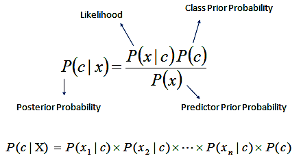
When there are multiple X variables, we simplify it by assuming that X’s are independent, so

For n number of X, the formula becomes Naive Bayes:

Which can be expressed as:

Since the denominator is constant here so we can remove it. It’s purely your choice if you want to remove it or not. Removing the denominator will help you save time and calculations.

This formula can also be understood as:
There are a whole lot of formulas mentioned here but worry not we will try to understand all this with the help of an example.
Naive Bayes Example
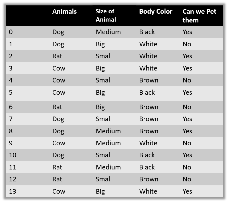
Let’s take a dataset to predict whether we can pet an animal or not.
Assumptions of Naive Bayes
· All the variables are independent. That is if the animal is Dog that doesn’t mean that Size will be Medium
· All the predictors have an equal effect on the outcome. That is, the animal being dog does not have more importance in deciding If we can pet him or not. All the features have equal importance.
We should try to apply the Naive Bayes formula on the above dataset however before that, we need to do some precomputations on our dataset.
We need to find P(xi|yj) for each xi in X and each yj in Y. All these calculations have been demonstrated below:
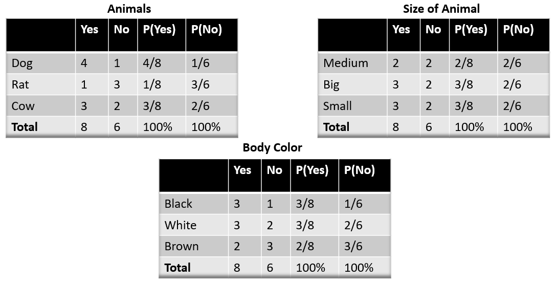
Image Source: Author
We also need the probabilities (P(y)), which are calculated in the table below. For example, P(Pet Animal = NO) = 6/14.

Now if we send our test data, suppose test = (Cow, Medium, Black)
Probability of petting an animal :


And the probability of not petting an animal:


We know P(Yes|Test)+P(No|test) = 1
So, we will normalize the result:
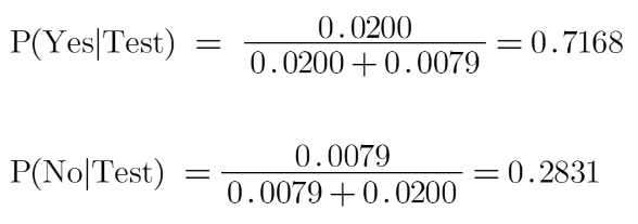
We see here that P(Yes|Test) > P(No|Test), so the prediction that we can pet this animal is “Yes”.
Gaussian Naive Bayes
So far, we have discussed how to predict probabilities if the predictors take up discrete values. But what if they are continuous? For this, we need to make some more assumptions regarding the distribution of each feature. The different naive Bayes classifiers differ mainly by the assumptions they make regarding the distribution of P(xi | y). Here we’ll discuss Gaussian Naïve Bayes.
Gaussian Naïve Bayes is used when we assume all the continuous variables associated with each feature to be distributed according to Gaussian Distribution. Gaussian Distribution is also called Normal distribution.
The conditional probability changes here since we have different values now. Also, the (PDF) probability density function of a normal distribution is given by:

We can use this formula to compute the probability of likelihoods if our data is continuous.
Frequently Asked Questions
A. The Naive Bayes algorithm is used due to its simplicity, efficiency, and effectiveness in certain types of classification tasks. It’s particularly suitable for text classification, spam filtering, and sentiment analysis. It assumes independence between features, making it computationally efficient with minimal data. Despite its “naive” assumption, it often performs well in practice, making it a popular choice for various applications.
A. The Naive Bayes algorithm is a probabilistic classification technique based on Bayes’ theorem. It assumes that all features in the data are independent of each other, given the class label. It calculates the probability of a particular class for a given set of features and selects the class with the highest probability as the predicted class. It’s commonly used in text classification and spam filtering tasks.
Endnotes
Naive Bayes algorithms are mostly used in face recognition, weather prediction, Medical Diagnosis, News classification, Sentiment Analysis, etc. In this article, we learned the mathematical intuition behind this algorithm. You have already taken your first step to master this algorithm and from here all you need is practice.
Did you find this article helpful? Please share your opinions/thoughts in the comments section below.
About the Author
I am an undergraduate student currently in my last year majoring in Statistics (Bachelors of Statistics) and have a strong interest in the field of data science, machine learning, and artificial intelligence. I enjoy diving into data to discover trends and other valuable insights about the data. I am constantly learning and motivated to try new things.
I am open to collaboration and work.
For any doubt and queries, feel free to contact me on Email
Connect with me on LinkedIn and Twitter
The media shown in this article are not owned by Analytics Vidhya and are used at the Author’s discretion.


