I recently completed a course on NLP through Deep Learning (CS224N) at Stanford and loved the experience. Learnt a whole bunch of new things. For my final project I worked on a question answering model built on Stanford Question Answering Dataset (SQuAD). In this blog, I want to cover the main building blocks of a question answering model.

You can find the full code on my Github repo.
I have also recently added a web demo for this model where you can put in any paragraph and ask questions related to it. Check it out at link
SQuAD Dataset
Stanford Question Answering Dataset (SQuAD) is a new reading comprehension dataset, consisting of questions posed by crowdworkers on a set of Wikipedia articles, where the answer to every question is a segment of text, or span, from the corresponding reading passage. With 100,000+ question-answer pairs on 500+ articles, SQuAD is significantly larger than previous reading comprehension datasets.
There has been a rapid progress on the SQuAD dataset with some of the latest models achieving human level accuracy in the task of question answering!
Examples of context, question and answer on SQuAD
Context — Apollo ran from 1961 to 1972, and was supported by the two-man Gemini program which ran concurrently with it from 1962 to 1966. Gemini missions developed some of the space travel techniques that were necessary for the success of the Apollo missions. Apollo used Saturn family rockets as launch vehicles. Apollo/Saturn vehicles were also used for an Apollo Applications Program, which consisted of Skylab, a space station that supported three manned missions in 1973–74, and the Apollo–Soyuz Test Project, a joint Earth orbit mission with the Soviet Union in 1975.
Question — What space station supported three manned missions in 1973–1974?
Answer — Skylab
Key Features of SQuAD:
i) It is a closed dataset meaning that the answer to a question is always a part of the context and also a continuous span of context
ii) So the problem of finding an answer can be simplified as finding the start index and the end index of the context that corresponds to the answers
iii) 75% of answers are less than equal to 4 words long
Machine Comprehension Model — Key Components
i) Embedding Layer
The training dataset for the model consists of context and corresponding questions. Both of these can be broken into individual words and then these words converted into Word Embeddings using a pre-trained vector like GloVevectors. To learn more about Word Embeddings please check out this article from me. Word Embeddings are much better at capturing the context around the words than using one hot vector for every word. For this problem I used 100 dimension GloVe word embeddings and didn’t tune them during the training process since we didn’t have sufficient data.
ii) Encoder Layer

The next layer we add in the model is an RNN based Encoder layer. We would like each word in the context to be aware of words before it and after it. A bi-directional GRU/LSTM can help do that. The output of the RNN is a series of hidden vectors in the forward and backward direction and we concatenate them. Similarly, we can use the same RNN Encoder to create question hidden vectors.
iii) Attention Layer
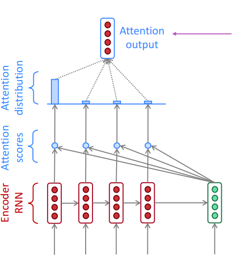
Up until now, we have a hidden vector for context and a hidden vector for the question. To figure out the answer we need to look at the two together. This is where attention comes in. It is the key component in the Question Answering system since it helps us decide, given the question which words in the context should I “attend” to. Let’s start with the simplest possible attention model:
Dot product attention

The dot product attention would be that for each context vector c i we multiply each question vector q j to get vector e i (attention scores in the figure above). Then we take a softmax over e i to get α i(attention distribution in the figure above). Softmax ensures that the sum of all e i is 1. Finally we calculate a i as the product of the attention distribution α i and the corresponding question vector(attention output in the figure above). Dot product attention is also described in the equations below
The above attention has been implemented as baseline attention in the Github code.
More Complex Attention — BiDAF Attention
You can run the SQuAD model with the basic attention layer described above but the performance would not be good. More complex attention leads to much better performance.
Lets describe the attention in the BiDAF paper. The main idea is that attention should flow both ways — from the context to the question and from the question to the context.
We first compute the similarity matrix S ∈ R N×M, which contains a similarity score Sij for each pair (ci , qj ) of context and question hidden states. Sij = wT sim[ci ; qj ; ci ◦ qj ] ∈ R Here, ci ◦ qj is an elementwise product and wsim ∈ R 6h is a weight vector. Described in equation below:
Next, we perform Context-to-Question (C2Q) Attention. (This is similar to the dot product attention described above). We take the row-wise softmax of S to obtain attention distributions α i , which we use to take weighted sums of the question hidden states q j , yielding C2Q attention outputs a i .
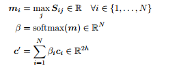
Next, we perform Question-to-Context(Q2C) Attention. For each context location i ∈ {1, . . . , N}, we take the max of the corresponding row of the similarity matrix, m i = max j Sij ∈ R. Then we take the softmax over the resulting vector m ∈ R N — this gives us an attention distribution β ∈ R N over context locations. We then use β to take a weighted sum of the context hidden states c i — this is the Q2C attention output c prime. See equations below
Finally for each context position c i we combine the output from C2Q attention and Q2C attention as described in the equation below
If you found this section confusing, don’t worry. Attention is a complex topic. Try reading the BiDAF paper with a cup of tea 🙂
iv) Output Layer
Almost there. The final layer of the model is a softmax output layer that helps us decide the start and the end index for the answer span. We combine the context hidden states and the attention vector from the previous layer to create blended reps. These blended reps become the input to a fully connected layer which uses softmax to create a p_start vector with probability for start index and a p_end vector with probability for end index. Since we know that most answers the start and end index are max 15 words apart, we can look for start and end index that maximize p_start*p_end.
Our loss function is the sum of the cross-entropy loss for the start and end locations. And it is minimized using Adam Optimizer.
The final model I built had a bit more complexity than described above and got to a F1 score of 75 on the test set. Not bad!
Next Steps
Couple of additional ideas for future exploration:
- I have been experimenting with a CNN based Encoder to replace the RNN Encoder described since CNNs are much faster than RNNs and more easy to parallelize on a GPU
- Additional attention mechanisms like Dynamic Co-attention as described in the paper
Give me a ❤️ if you liked this post:) Hope you pull the code and try it yourself.
Other writings: http://deeplearninganalytics.org/blog
PS: I have my own deep learning consultancy and love to work on interesting problems. I have helped several startups deploy innovative AI based solutions. Check us out at — http://deeplearninganalytics.org/.
If you have a project that we can collaborate on, then please contact me through my website or at priya.toronto3@gmail.com
References:


