In this article, we will use a dataset to understand how to build different classification models in python from scratch. The models that will be introduced in this article are,
- Logistic Regression
- Decision Trees
- Random Forest
- K nearest neighbor.
After we build the models using training data, we will test the accuracy of the model with test data and determine the appropriate model for this dataset.
For this exercise, I have used Jupyter Notebook.
The dataset used is available on Kaggle – Heart Attack Prediction and Analysis
In this article, we will focus only on implementing outlier detection, outlier treatment, training models, and choosing an appropriate model.
Problem Statement:
Age : Age of the patient
Sex : Sex of the patient
exang: exercise induced angina (1 = yes; 0 = no)
ca: number of major vessels (0-3)
cp : Chest Pain type chest pain type
Value 1: typical angina
Value 2: atypical angina
Value 3: non-anginal pain
Value 4: asymptomatic
trtbps : resting blood pressure (in mm Hg)
chol : cholestoral in mg/dl fetched via BMI sensor
fbs : (fasting blood sugar > 120 mg/dl) (1 = true; 0 = false)
rest_ecg : resting electrocardiographic results
Value 0: normal
Value 1: having ST-T wave abnormality (T wave inversions and/or ST elevation or depression of > 0.05 mV)
Value 2: showing probable or definite left ventricular hypertrophy by Estes’ criteria
thalach: maximum heart rate achieved
output: 0= less chance of heart attack 1= more chance of heart attack
Before we start with code, we need to import all the required libraries in Python.
I follow a convention of dedicating one cell in the Notebook only for imports. This is beneficial when we want to add additional import statements. We just need to run the cell which only has imports. It will not affect the remaining ‘code’.
Python Code:
Before proceeding, we will get a basic understanding of our data by using the following command.
data1.info()
Now, we want to understand the number of records and the number of features. This can be achieved by using the following code snippet,
#number of records and features in the dataset
data1.shape
The 303 in the output defines the number of records in the dataset and 14 defines the number of features in the dataset including the ‘target variable’.
Data Cleaning/ Data preprocessing
Before providing data to a model, it is essential to clean the data and treat the nulls, outliers, duplicate data records.
We will begin with checking for duplicate rows with the code snippet,
#Check duplicate rows in data
duplicate_rows = data1[data1.duplicated()]
print("Number of duplicate rows :: ", duplicate_rows.shape)
The data contains 1 duplicate row. We will remove the duplicate row and check for duplicates again.
#we have one duplicate row.
#Removing the duplicate row
data1 = data1.drop_duplicates()
duplicate_rows = data1[data1.duplicated()]
print("Number of duplicate rows :: ", duplicate_rows.shape)
#Number of duplicate rows after dropping one duplicate row
Now, there are 0 duplicate rows in the data. We will check for ‘null’ values in the data.
#Looking for null values
print("Null values :: ")
print(data1.isnull() .sum())
#Check if the other data is consistent
data1.shape
As there are no ‘null’ values in data, we will go ahead with ‘Outlier Detection‘ using box plots.
We will plot box plots for all features.
#As there are no null values in data, we can proceed with the next steps.
#Detecting Outliers
# 1. Detecting Outliers using IQR (InterQuartile Range)
sns.boxplot(x=data1['age'])
#No Outliers observed in 'age'
sns.boxplot(x=data1['sex'])
#No outliers observed in sex data
sns.boxplot(x=data1['cp'])
#No outliers in 'cp'
sns.boxplot(x=data1['trtbps'])
#Some outliers are observed in 'trtbps'. They will be removed later
sns.boxplot(x=data1['chol'])
#Some outliers are observed in 'chol'. They will be removed later
sns.boxplot(x=data1['fbs'])
sns.boxplot(x=data1['restecg'])
sns.boxplot(x=data1['thalachh'])
#Outliers present in thalachh
sns.boxplot(x=data1['exng'])
sns.boxplot(x=data1['oldpeak'])
#Outliers are present in 'OldPeak'
sns.boxplot(x=data1['slp'])
sns.boxplot(x=data1['caa'])
#Outliers are present in 'caa'
sns.boxplot(x=data1['thall'])
From the box plots, outliers are present in trtbps, chol, thalachh, oldpeak, caa, thall.
The Outliers are removed using two methods,
1. Inter-Quartile Range and
2. Z-score
We will use both methods and check the effect on the dataset.
1. Inter-Quartile Range
In IQR, the data points higher than the upper limit and lower than the lower limit are considered outliers.
- upper limit = Q3 + 1.5 * IQR
- lower limit = Q1 – 1.5 * IQR
We find the IQR for all features using the code snippet,
#Find the InterQuartile Range
Q1 = data1.quantile(0.25)
Q3 = data1.quantile(0.75)
IQR = Q3-Q1
print('*********** InterQuartile Range ***********')
print(IQR)
# Remove the outliers using IQR
data2 = data1[~((data1<(Q1-1.5*IQR))|(data1>(Q3+1.5*IQR))).any(axis=1)]
data2.shape
After removing outliers using IQR, the data contains 228 records.
2. Z – Score
If a Z-score is greater than 3, it implies that the data point differs from the other data points and hence is treated as an outlier.
#Removing outliers using Z-score
z = np.abs(stats.zscore(data1))
data3 = data1[(z<3).all(axis=1)]
data3.shape
After using Z-score to detect and remove outliers, the number of records in the dataset is 287.
As the number of records available is higher after Z-score, we will proceed with ‘data3’
Correlation
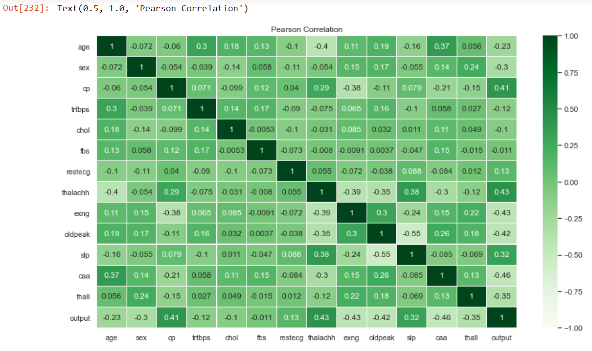
After removing outliers from data, we will find the correlation between all the features.
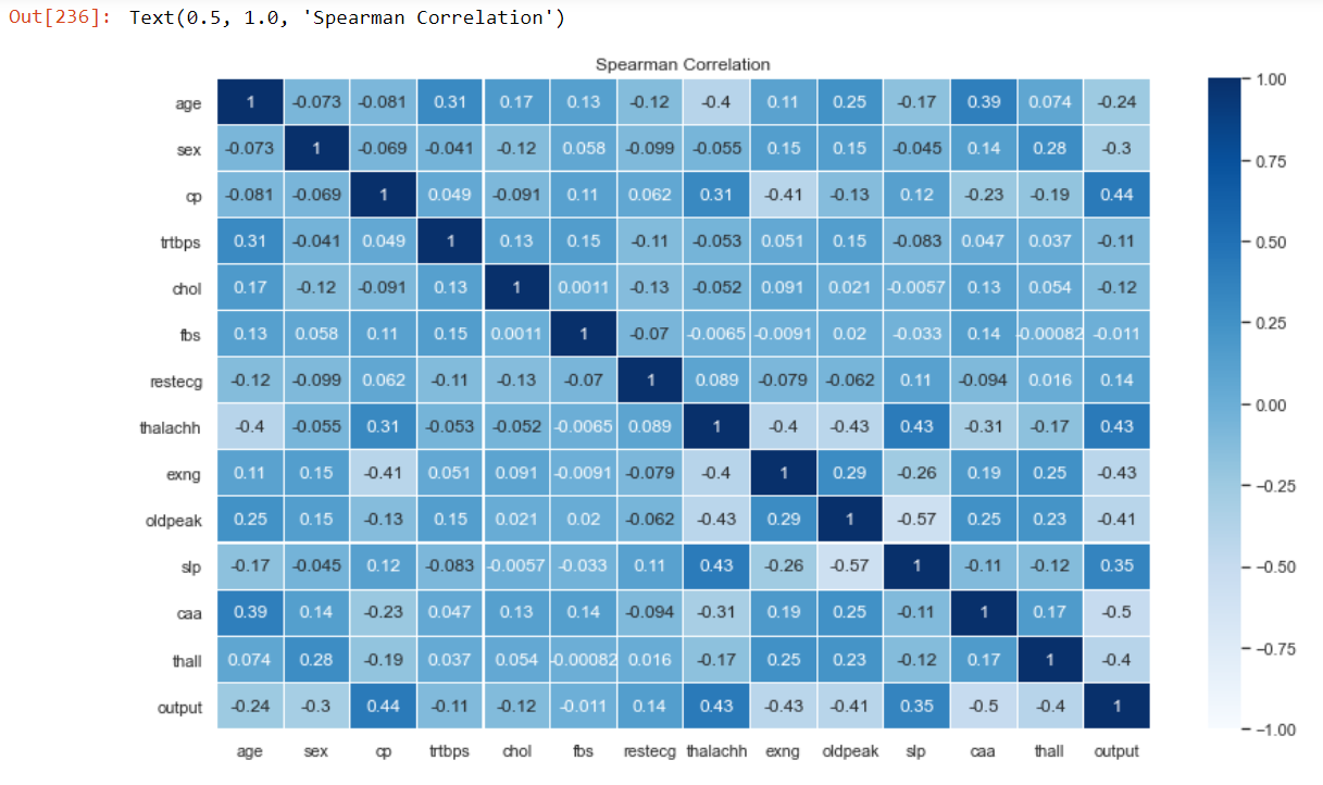
Two types of correlation will be used here.
- Pearson Correlation
- Spearman Correlation
1. Pearson Correlation
#Finding the correlation between variables
pearsonCorr = data3.corr(method='pearson')
spearmanCorr = data3.corr(method='spearman')
fig = plt.subplots(figsize=(14,8))
sns.heatmap(pearsonCorr, vmin=-1,vmax=1, cmap = "Greens", annot=True, linewidth=0.1)
plt.title("Pearson Correlation")

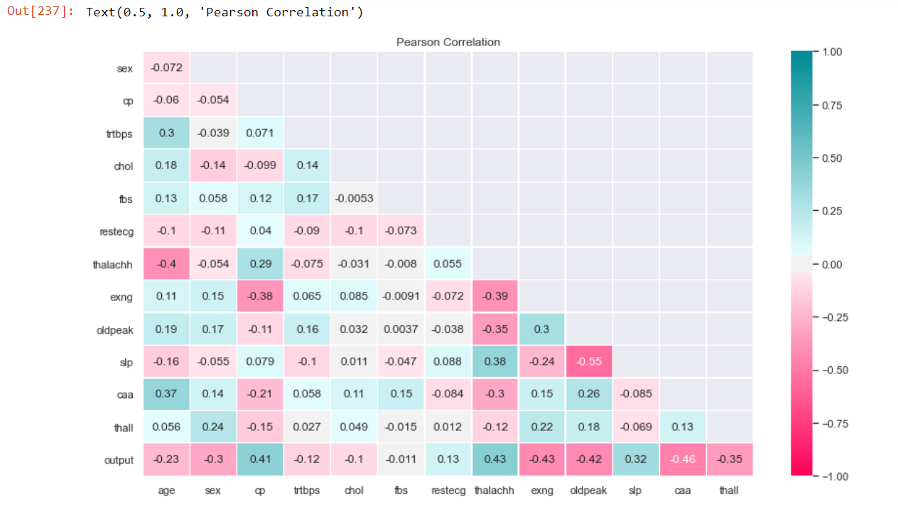
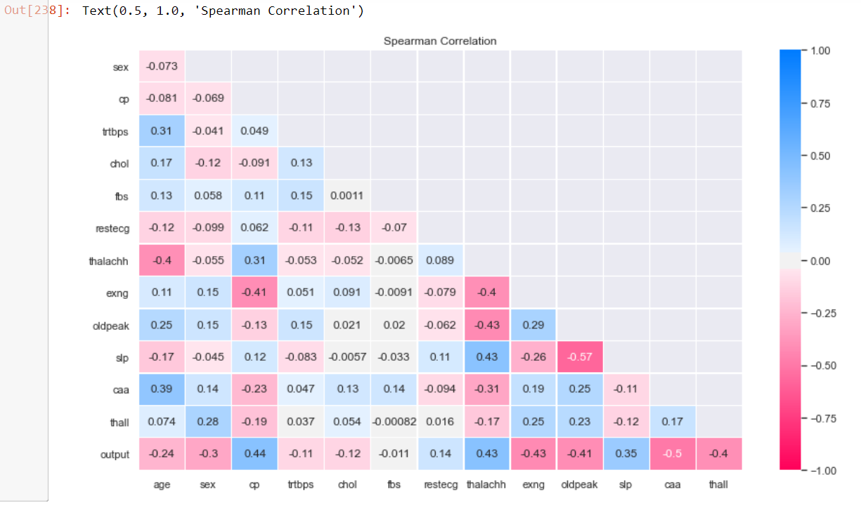
From the heat map, the same values of correlation are repeated twice. To remove this, we will mask the upper half of the heat map and show only the lower half. The same procedure will be carried out for Spearman Correlation.
#Create mask for both correlation matrices
#Pearson corr masking
#Generating mask for upper triangle
maskP = np.triu(np.ones_like(pearsonCorr,dtype=bool))
#Adjust mask and correlation
maskP = maskP[1:,:-1]
pCorr = pearsonCorr.iloc[1:,:-1].copy()
#Setting up a diverging palette
cmap = sns.diverging_palette(0, 200, 150, 50, as_cmap=True)
fig = plt.subplots(figsize=(14,8))
sns.heatmap(pCorr, vmin=-1,vmax=1, cmap = cmap, annot=True, linewidth=0.3, mask=maskP)
plt.title("Pearson Correlation")

2. Spearman Correlation
fig = plt.subplots(figsize=(14,8))
sns.heatmap(spearmanCorr, vmin=-1,vmax=1, cmap = "Blues", annot=True, linewidth=0.1)
plt.title("Spearman Correlation")

After masking the upper half of the heat map,
#Create mask for both correlation matrices
#Spearson corr masking
#Generating mask for upper triangle
maskS = np.triu(np.ones_like(spearsonCorr,dtype=bool))
#Adjust mask and correlation
maskS = maskS[1:,:-1]
sCorr = spearsonCorr.iloc[1:,:-1].copy()
#Setting up a diverging palette
cmap = sns.diverging_palette(0, 250, 150, 50, as_cmap=True)
fig = plt.subplots(figsize=(14,8))
sns.heatmap(sCorr, vmin=-1,vmax=1, cmap = cmap, annot=True, linewidth=0.3, mask=maskS)
plt.title("Spearman Correlation")

From both the heat maps, the features fbps, chol and trtbps have the lowest correlation with output.
Classification
Before implementing any classification algorithm, we will divide our dataset into training data and test data. I have used 70% of the data for training and the remaining 30% will be used for testing.
#From this we observe that the minimum correlation between output and other features in
#fbs,trtbps and chol
x = data3.drop("output", axis=1)
y = data3["output"]
x_train,x_test,y_train,y_test = train_test_split(x,y,test_size=0.3)
We will implement four classification algorithms,
1. Logistic Regression Classifier
2. Decision Trees Classifier
3. Random Forest Classifier
4. K Nearest Neighbours Classifier
1. Logistic Regression Classifier
The code snippet used to build Logistic Regression Classifier is,
#Building classification models
names = ['Age', 'Sex', 'cp', 'trtbps', 'chol', 'fbs', 'restecg', 'thalachh', 'exng', 'oldpeak', 'slp', 'caa', 'thall']
#   ****************Logistic Regression*****************
logReg = LogisticRegression(random_state=0, solver='liblinear')
logReg.fit(x_train, y_train)
#Check accuracy of Logistic Regression
y_pred_logReg = logReg.predict(x_test)
#Model Accuracy
print("Accuracy of logistic regression classifier :: " ,metrics.accuracy_score(y_test,y_pred_logReg))
#Removing the features with low correlation and checking effect on accuracy of model
x_train1 = x_train.drop("fbs",axis=1)
x_train1 = x_train1.drop("trtbps", axis=1)
x_train1 = x_train1.drop("chol", axis=1)
x_train1 = x_train1.drop("restecg", axis=1)
x_test1 = x_test.drop("fbs", axis=1)
x_test1 = x_test1.drop("trtbps", axis=1)
x_test1 = x_test1.drop("chol", axis=1)
x_test1 = x_test1.drop("restecg", axis=1)
logReg1 = LogisticRegression(random_state=0, solver='liblinear').fit(x_train1,y_train)
y_pred_logReg1 = logReg1.predict(x_test1)
print("nAccuracy of logistic regression classifier after removing features:: " ,metrics.accuracy_score(y_test,y_pred_logReg1))
The accuracy of logistic regression classifier using all features is 85.05%
While the accuracy of logistic regression classifier after removing features with low correlation is 88.5%
2. Decision Tree Classifier
The code snippet used to build a decision tree is,
# ***********************Decision Tree Classification***********************
decTree = DecisionTreeClassifier(max_depth=6, random_state=0)
decTree.fit(x_train,y_train)
y_pred_decTree = decTree.predict(x_test)
print("Accuracy of Decision Trees :: " , metrics.accuracy_score(y_test,y_pred_decTree))
#Remove features which have low correlation with output (fbs, trtbps, chol)
x_train_dt = x_train.drop("fbs",axis=1)
x_train_dt = x_train_dt.drop("trtbps", axis=1)
x_train_dt = x_train_dt.drop("chol", axis=1)
x_train_dt = x_train_dt.drop("age", axis=1)
x_train_dt = x_train_dt.drop("sex", axis=1)
x_test_dt = x_test.drop("fbs", axis=1)
x_test_dt = x_test_dt.drop("trtbps", axis=1)
x_test_dt = x_test_dt.drop("chol", axis=1)
x_test_dt = x_test_dt.drop("age", axis=1)
x_test_dt = x_test_dt.drop("sex", axis=1)
decTree1 = DecisionTreeClassifier(max_depth=6, random_state=0)
decTree1.fit(x_train_dt, y_train)
y_pred_dt1 = decTree1.predict(x_test_dt)
print("Accuracy of decision Tree after removing features:: ", metrics.accuracy_score(y_test,y_pred_dt1))
The accuracy of the decision tree with all features is 70.11% while accuracy after removing low correlation features is 78.16%
3. Random Forest Classifier
Implement a random forest classifier using the code,
# Using Random forest classifier
rf = RandomForestClassifier(n_estimators=500)
rf.fit(x_train,y_train)
y_pred_rf = rf.predict(x_test)
print("Accuracy of Random Forest Classifier :: ", metrics.accuracy_score(y_test, y_pred_rf))
#Find the score of each feature in model and drop the features with low scores
f_imp = rf.feature_importances_
for i,v in enumerate(f_imp):
    print('Feature: %s, Score: %.5f' % (names[i],v))
The accuracy of the model is 86.20%. Along with accuracy, we will also print the feature and its importance in the model. Then, we will eliminate features with low importance and create another classifier and check the effect on the accuracy of the model. As all the features have some contribution to the model, we will keep all the features.
4. K Nearest Neighbours Classifier
Implement K nearest neighbor classifier and print the accuracy of the model.
#K Neighbours Classifier
knc =  KNeighborsClassifier()
knc.fit(x_train,y_train)
y_pred_knc = knc.predict(x_test)
print("Accuracy of K-Neighbours classifier :: ", metrics.accuracy_score(y_test,y_pred_knc))
The accuracy is only 59.77%
Conclusion
#Models and their accuracy
print("*****************Models and their accuracy*****************")
print("Logistic Regression Classifier :: ", metrics.accuracy_score(y_test,y_pred_logReg1))
print("Decision Tree :: ", metrics.accuracy_score(y_test,y_pred_dt1))
print("Random Forest Classifier :: ", metrics.accuracy_score(y_test, y_pred_rf))
print("K Neighbours Classifier :: ", metrics.accuracy_score(y_test,y_pred_knc))
After implementing four classification models and comparing their accuracy, we can conclude that for this dataset Logistic Regression Classifier is the appropriate model to be used.
About Me:
Data Visualization Enthusiast. Business Analytics Student. E&TC Engineer.
LinkedIN: https://www.linkedin.com/in/kothadiashruti/
Medium: https://kothadiashruti.medium.com/
Kaggle Notebook link for entire code.
The media shown in this article are not owned by Analytics Vidhya and is used at the Author’s discretion.


