Classifying DDoS attacks with Artificial Intelligence

Introduction

The majority of corporates or services rely highly upon networking infrastructure which supports core functionalities of IT operations for the organization. Therefore the health of the networking infrastructure should always be kept intact and monitored for any possible issues that may pop up any sooner or later.

The purpose of monitoring is not only limited to hardware faults or the bugs in embedded software but could also be applied to take care of security vulnerabilities or if not at least to avoid possible attacks.

The networking infrastructure though secured mostly suffers from the bot and DDoS attacks which are usually not detected as suspicious since they target the resource allocation system of the network devices which could be normal in some cases of heavy utilization.

Well, there is a catch for this, most of the time this resource allocation is not likely to cause storms in multiple devices and hence could easily be tracked through the time domain to detect any anomalies. Most modern firewalls can detect the requests coming in a suspicious manner by a number of SYN, ICMP connection requests in a second, but this still doesn’t provide any conclusion. Now when we get inside the anomalies, we can uncover a pattern that must have been triggered by the action of the attacker’s request. This pattern could be a power consumption of the device, CPU utilization, memory, and anything.

As I say to you the anomalies, the first thing that comes to mind is Artificial Intelligence and Machine Learning. Machine Learning is a discipline of AI that aids machines or computers to learn from history and then use it to predict the outcome with enough accuracy which should suffice the purpose. Machine learning identifies the statistical patterns at the smallest possible levels that are responsible for that specific outcome (attack in this case), then associates that reaction for further references. This is how it helps us predict the outcomes.

Background of DDoS attacks:

DDoS attacks are very common.DDoS attacks are a dominant threat to the vast majority of service providers — and their impact is widespread. These attacks represent up to 25 percent of a country’s total Internet traffic while they are occurring.

Organizations are spending anywhere from thousands to millions of dollars on securing their infrastructure against these threats, yet they are compromised due to the fact that These attacks tend to stay throughput on sending requests which will eventually keep the resources busy on the device till the device hangs up just like when your computer gets crashed due to heavy loads. The resources utilized by the attacks could be memory, CPU or NVRAM, or network congestion. The motive of DDoS attacks may not be to penetrate the network to steal information but to disrupt the network flow enough to cause the company to incur heavy losses.

Creepy ha! Nah it’s a loophole in our model which has to be identified.

Mechanism of attack:

There are many types of attacks like IMPS flooding, Ping Death, UDP flooding, and all have one thing in common, that is to send a number of requests to keep the device or traffic channel saturated.

The DDoS attack is initialized by an attacker through a computer that will start sending requests or update a malicious application on other devices to utilize them as a bot which helps attack spread and make it difficult to mitigate. The mitigation cases could take a long time as the compromised network needs to release all the requests being sent by identified devices.

I will leave links to the summary of the types of DDoS attacks here if you want to learn more.

https://www.cloudflare.com/learning/ddos/what-is-a-ddos-attack/

How does machine learning help?

The tools like Statseeker, NNM are used for monitoring devices which show up a graph that is very simple to check and conclude the status. The same concept can be used to collect data points and run them through a trained machine learning model to check for any anomalies at smaller discrete scales. But first, we need to teach our model and find the most common patterns that were associated with the initial phase of the attack. Likewise, we need a dataset that has either been collected from the actual attack or simulated attacks in a test space. Then we will proceed to train and test our model.

Implementation:

The main independent in detecting DDoS attacks is the pack and bit flow per second. To do so we need some dataset form, then processing it to match our requirements.

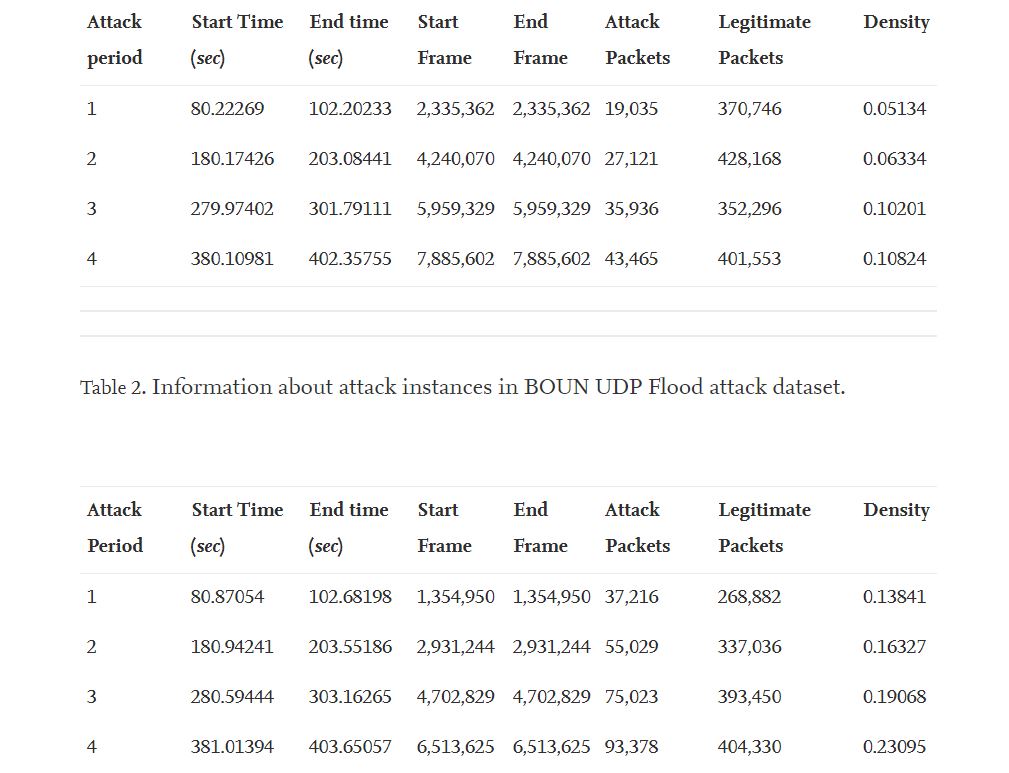
I have chosen Dataset from Boğaziçi University Experiment which you can find in the link along with a detailed description of the dataset. This is very simple to understand the concept and implementation. The data collected here is through the network setup tracked down by the Wireshark and exported as CSV files. There are two files available separately for TCP-SYN and UDP attacks respectively.

Link for the article :

https://www.sciencedirect.com/science/article/pii/S2352340920310817#bib0005

Link for downloading a dataset :

http://dx.doi.org/10.17632/mfnn9bh42m.1#file-ba7d3a46-1dc3-452e-aeac-26d909389b29

Though the dataset has most components already still, I was required to do some manual work to tweak it to feature selection.

To begin I first imported the downloaded dataset, Extracted the designated rows of attacks Manually Labelled the rows as mentioned in the Journal article to separate the Attack session from normal traffic. Then merged all datasets into a single file.

Source: Sciencedirect

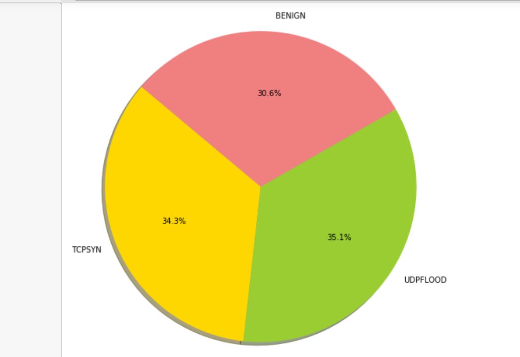
The Attack Types included are TCP-SYN, UDP Flood, and normal traffic are named Benign.

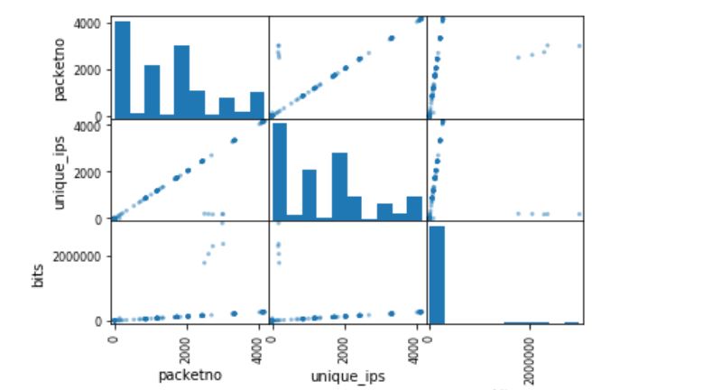
The TCP-SYN and UDP floods can be identified by high packet and bit flow along with a considerable number of unique IPs which indicates spoofing.

The Benign or normal traffic on another hand even if has a high packet or bit rate, still will have less no. of IP addresses added in-memory table.

So patterns above help us select the features for our model.

To process dataset first I took columns “Time”,”Attack”,”Source_ip”,’Frame_length’

The time column is used to get Set of IP addresses, packets, and byte length per second by iterating through each row till we find the next second of time.

The attack is used as a label for each attack/traffic type, Source_ip to track down the number of unique IP requests per second which is especially useful in the case of TCP SYN as a three-way handshake takes place.

Frame_length denotes the length of the frame in bytes which would be iterated over rows and added up till the next second of time.

Then after processing, we have one more dataset that actually is free from unnecessary errors, null values, and large datatypes consuming memory.

Also, note that depending on the availability of memory you may have to convert some columns to different data types to narrow through down-casting. In my case, I did for a time as there was no need for high precision since I had scaled to seconds and converted to 32-bit unsigned integer.

Code:

Import required libraries:

from pandas import read_csv
from pandas.plotting import scatter_matrix
from matplotlib import pyplot
from sklearn.model_selection import train_test_split
from sklearn.model_selection import cross_val_score
from sklearn.model_selection import StratifiedKFold
from sklearn.metrics import classification_report
from sklearn.metrics import confusion_matrix
from sklearn.metrics import accuracy_score
from sklearn.tree import DecisionTreeClassifier
from sklearn.neighbors import KNeighborsClassifier
from sklearn.discriminant_analysis import LinearDiscriminantAnalysis
import numpy as np
import seaborn as sns
from pandas import DataFrame

file2 = r"mfnn9bh42m-1BOUN_DDoS datasetboun_tcp_Anon1.csv"
dataset = read_csv(file2, low_memory=False)
dataset = dataset[["Time","TTL","SYN","ACK","Attack","Source_ip",'Frame_length']]
dataset["SYN"] = dataset["SYN"].fillna(0)
fataset["ACK"] = dataset["ACK"].fillna(0)
dataset["SYN"] = dataset["SYN"].replace(['Set','Not set'],[1,0])
dataset["ACK"] = dataset["ACK"].replace(['Set','Not set'],[1,0])
dataset["Time"] = dataset["Time"].fillna(0)

#dataset["Attack_type"] = dataset["Attack_type"].fillna("BENIGN")
dataset["Time"] = dataset["Time"].astype(np.uint32)
S=[]
packetno = 1
M=[]
bits = 0

for i in range(1,len(dataset)):
      if dataset.loc[i,'Time']>=(dataset.loc[i-1,'Time'])+1 or dataset.loc[i,'Attack']!=dataset.loc[i-1,'Attack']: 
              M = set(M)
              unique_ips = len(M)
              Attack_type = dataset.loc[i,"Attack"]
              S.append([packetno,unique_ips,bits,Attack_type])
              packetno = 0
              bits = 0
              M = []
       else:
             bits += dataset.loc[i,'Frame_length']
             M.append(dataset.loc[i,'Source_ip'])
             packetno += 1
             S.append([packetno,unique_ips,bits,Attack_type])
             S = DataFrame(S,columns = ['packetno','unique_ips','bits','Attack_type'])
             S = S.dropna()
             print(S)
             print(S.describe())
             print(S.groupby("Attack_type").size())

Distribution of Data, well I had a bit of an issue distributing it equally.

Visualizing the Dataset through Pie Chart:

import matplotlib.pyplot as plt
labels = 'TCPSYN','UDPFLOOD','BENIGN'
sizes = [len(S[S["Attack_type"]=="TCPSYN"]),len(S[S["Attack_type"]=="UDPFLOOD"]),len(S[S["Attack_type"]=="BENIGN"])]
colors = ['gold', 'yellowgreen', 'lightcoral', 'lightskyblue','yellow','purple','grey']
explode = (0, 0, 0) # explode 1st slice

# Plot
plt.rcParams.update({'font.size': 10})
plt.figure(figsize=(8,8))
plt.pie(sizes, explode=explode, labels=labels, colors=colors,
autopct='%1.1f%%', shadow=True, startangle=140)
plt.axis('equal')
plt.show()

scatter_matrix(S)
pyplot.show()

Training the Models with different algorithms:

While some algorithms may not be suitable for this application, I have excluded Logistic Regression and SVM.

# Spot Check Algorithms
models = []
models.append(('LDA', LinearDiscriminantAnalysis()))
models.append(('KNN', KNeighborsClassifier()))
models.append(('CART', DecisionTreeClassifier()))
models.append(('NB', GaussianNB()))

# evaluate each model in turn
results = []
names = []
for name, model in models:
kfold = StratifiedKFold(n_splits=10, random_state=1, shuffle=True)
cv_results = cross_val_score(model, X_train, Y_train, cv=kfold, scoring='accuracy')
results.append(cv_results)
names.append(name)
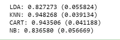
print('%s: %f (%f)' % (name, cv_results.mean(), cv_results.std()))

Results:

Improvements:

The accuracy highly relies upon the features selected and it can be analyzed by some methods like Correlation coefficient, Chi-square test, information gain analysis ( which I prefer).

Adding some more features like RST, SYN, SYN-ACK bit reading can improve the classifier but will high-end machines or VM platforms deployed over the cloud (Azure or AWS, Digital ocean) since the attribute list becomes complex and very bulky. The training may also require a high-performance CPU/GPU and a good amount of memory.

The accuracy can be increased by identifying more patterns and features either through a larger dataset or unsupervised learning implemented by Tensorflow.

there is an open-source library for python called “pyshark” which can be used to log live data and use it directly inside the application that implements the classifier.

The model can be tested live in a test environment to check the detection and classification accuracy.

I have plans to workout unsupervised learning and back it up with live data coming from pyshark as stated above.

Pannag S

06 Apr 2021