This article was published as a part of the Data Science Blogathon.
Introduction
Isotonic Regression is one of those regression technique that is less talked about but surely one of the coolest ones. I say “less talked about” because unlike linear regression it is not taught frequently or used. Isotonic Regression makes a more general, weaker assumption that the function that represents the data best is monotone rather than linear(yes, linear is also monotone but not a vice, versa).
The word “Isotonic” originates from two Greek root words: “iso” and “tonos“; “iso” literally meaning equal and “tonos” meaning to stretch. Thus Isotonic Regression, also called Equal Stretch Regression, fits a piecewise-constant non-decreasing(step-like) function to the data and hence provides an alternative to linear regression, which essentially fits a straight line to the data.
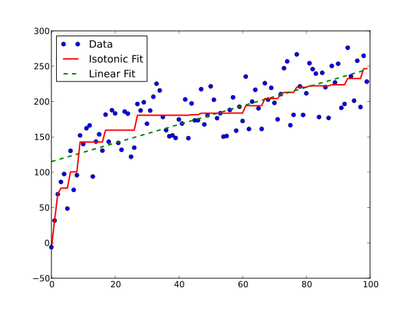
Here’s what Isotonic Regression looks like in comparison to Linear regression.
If you are like me then you probably like to know the maths behind algorithms before you can start using them. Knowing exactly what causes the algorithm to behave the way it does is a good practice for anyone who wishes to get the best results using it.
So here’s what we are going to do:
- Firstly, we will formulate the problem that Isotonic Regression solves.
- Then we will look at some math and try to understand the solution. In this part, we will encounter the PAVA algorithm.
- Lastly, we will look at its implementation in python and its main applications.
Problem formulation
Isotonic Regression solves the following problem: given a sequence of n data points y1,y2….yn, how can we best summarize this by a monotone sequence β1,….βn?

We will get back to this later. First, we need to formalize the monotone sequences. These sequences can be thought of in another way. We can divide the space in which the points lie into different sections depending upon the constraints. Then we can apply linear regression to the points present in the sections. This will give us an isotonic plot similar to the one present above.

To formulate the monotone sequences and what we mean by them, we have to make an assumption.
Homoscedastic Normal Errors
Like with other linear models we can assume that the errors in this type of regression are homoscedastic. In other words, all the errors will have finite variance. As the errors do not depend on the predictor values xi, we can formulate a linear model that can efficiently fit the data. Also, we can assume that the dependent variables are random and they follow a Normal distribution.

and

The above condition is due to the monotonicity constraints.
Dealing with Duplicate Predictor Values
We can see that when xi = xj implies μi = μj (same x values will have the same mean in the distribution of y).
So we can have one mean parameter for all duplicate predictor or x values, in other words, we can only have one mean parameter in y for each unique predictor or x value.
What does it even mean or why are we considering this in the first place? I mean how can we have duplicate x values?
I will explain one part of the question here, the other part requires some more explaining to do. So what do we mean by duplicate or same x values?
As we saw in the definition itself that Isotonic Regression fits the data in a monotonic manner. So while fitting the data, if the algorithm finds a point that violates this monotonicity constraint, the point is clubbed with adjacent x values to form a block or a monotone sequence that we considered earlier. The cool thing is that all the x values in a monotone sequence or block will have the same y value. You can see this in the isotonic curve present above where there are flat or stretched parts of the isotonic curves( yeah equal stretch regression gets its name from here).
These appear as steps in the plot. Now as to what will the value of y in these so-called blocks is what we are trying to find. You can probably see by now how the solution is reached by the PAVA algorithm. Now let’s find out exactly how the y values are calculated.
Let z1,….,zk be unique x values (which will have the same y value later) in sorted order.
Then we can define weights for all the unique x values as:-
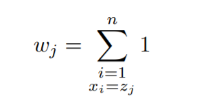
Therefore, now the dependent or y values become:-
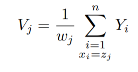
Now, as we are dividing the y values by their respective weights, the distribution of the y values will change to:-

Now, this distribution represents the unique y values that will be predicted, with components, v1,……,vk.
These components will be monotonic as it’s a constraint that we have to follow.

also,

Now we need to get back to the mathematical description.
Minus Log-Likelihood
You must have heard about maximum likelihood estimation in the case of linear regression and how it ultimately gives the line of best fit. Generally, we try to maximize the likelihood functions, but if we take the log of the likelihood function and multiply the whole expression by -1, what we get is the minus log-likelihood and it is to be minimized instead of maximizing due to the -1. So basically we are maximizing by minimizing.

We get this by taking the log of the Normal distribution(the distribution from which we assumed our y values came from) and multiplying by -1.
Lagrangian
If you know a thing or two about constrained optimization then chances are you have heard of the Lagrangian function. Whenever we are faced with the task of optimizing(here, minimizing) a cost function like we have above, with some constraints(here monotonicity), we take the help of Lagrange Multipliers.

The above equation is called the Lagrangian. Solving this equation will give us the minimum of the minus log-likelihood function and thus ultimately maximize the likelihood, ensuring the best fit to the data. Notice how an extra term is added in addition to the two already existing terms in the minus log-likelihood function. This extra term arises as a result of the constraints that we are taking into consideration. Hence making our problem a constrained optimization problem.
KKT Conditions
For an unconstrained convex optimization problem, we know that the minimum is achieved when the gradient is zero at a point. The KKT conditions are the equivalent conditions for the global minimum of a constrained convex optimization problem that we are facing now.
These conditions are namely:-
- Lagrangian minimization,
- Primal feasibility,
- Dual feasibility,
- Complementary slackness.
For the first condition(Lagrangian minimization),

Notice how we are taking the partial derivative of the Lagrangian with respect to the y values, or the values that are predicted.
Note that, ∂µi/∂νm is equal to 1 if xi = zm and 0 otherwise. So, the terms in the sum in the first line are non-zero only if xi = zm (where zm stands for the unique x values or the x values for which we will have unique y values).
As it can be seen, this formula is only valid for 1 < m < k. To make it valid for 1 <= m <= k, we define λ0 = λk = 0.
Setting the above equation to zero gives us the first Karush-Kuhn-Tucker condition. Let’s set it to zero and multiply by σ
2 throughout,

here κm = σ
2λm has been introduced.
It can be seen that κm is zero, positive, or negative exactly whenκm = σ 2λm is, therefore we can use κm in the rest of the KKT conditions.
Now the second condition (Primal feasibility):

for the third condition (Dual feasibility):

Lastly the (Complementary slackness) condition:

Now you may be wondering why have we introduced κm = σ 2λm . The reason is that while we are estimating the mean parameters or y values, in other words, we do not generally consider the variance. So as to carry out the maximum likelihood estimation without involving the variance we introduced a new variable that is only directly dependent on the Lagrange multipliers, λm.
Now that we have our KKT conditions, we are ready to finally compute the y values.
Defining Blocks
At first, we only apply the first(derivative of Lagrangian equal to zero) and fourth(complementary slackness) conditions.
We can divide the space of the y values into blocks of equal consecutive components and these blocks will have length one if the value in that block is not equal to the mean value on either side.
From this moment on, we will refer to the unique y values as ν, which is the mean of a particular block.
So let’s consider a block.
A block will have only one unique y value which we will refer to as v (mean parameter) in that block.
Suppose,

The asterisk in the superscript is used to differentiate two different blocks. Therefore the sequence, νj
∗ = · · · = νj
∗∗−1 represents a block.
Now for the edge cases, we define ν0 = −∞ and νk+1 = +∞.
The complementary slackness condition implies,

Therefore, now using the first condition we have,
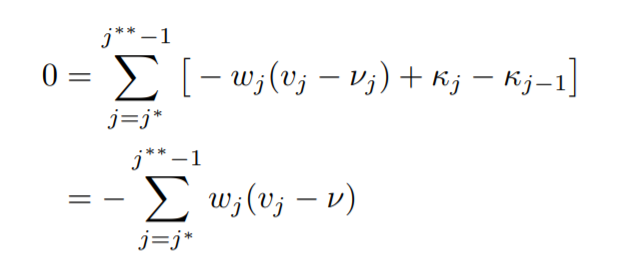
where,

Solving the above we get,

Now this reveals to us a piece of very important and cool information. By applying 1st and 4th conditions only, we find that,
the mean in a block of equal values is the weighted average of the vj values, which in turn is the unweighted average of the yi values for the block.
The Pool Adjacent Violators Algorithm(PAVA)
The PAVA algorithm basically does what its name suggests. It inspects the points and if it finds a point that violates the constraints, it pools that value with its adjacent members which ultimately go on to form a block.
Concretely PAVA does the following,
- [Initialization step] Set v and κ to any values satisfying conditions 1,3, and 4.
- [Termination Step] If condition 2 (primal condition) is satisfied, then terminate.
- [Pool Adjacent Violators] Choose any j such that νj > νj+1. And “pool” the blocks containing j and j + 1, that is, make
them one block (and the nu or µ values for this pooled block will again be the weighted average of the values
for this pooled block). [This step maintains conditions 1, 3, and 4.] - Go to Step 2 again.
Now that we have a basic idea of how this algorithm works, let’s implement it in python:
First, we need to import the required libraries:
import numpy as np
import pandas as pd
import matplotlib.pyplot as plt
from sklearn.linear_model import LinearRegression
from sklearn.isotonic import IsotonicRegression
from matplotlib.collections import LineCollection
import random
Then let’s generate some points and add some random noise to them:
Python Code:
Now let’s fit the data, linearly and isotonically,
ir=IsotonicRegression()
lr=LinearRegression()
y_ir=ir.fit_transform(x,y)
lr.fit(x[:,np.newaxis],y)
Generate some line segments and plot the results:
lines=[[[i,y[i]],[i,y_ir[i]]] for i in range(n)]
lc=LineCollection(lines)
plt.figure(figsize=(16,4))
plt.plot(x,y,'r.',markersize=12)
plt.plot(x,y_ir,'b.-',markersize=12)
plt.plot(x,lr.predict(x[:, np.newaxis]), 'y-')
plt.gca().add_collection(lc)
plt.legend(('Data','Isotonic Fit','Linear Fit'))
plt.title("Isotonic Regression")
Final Result:

One can also see the algorithm working in real-time:
Applications
Now the question becomes, where is Isotonic Regression used?
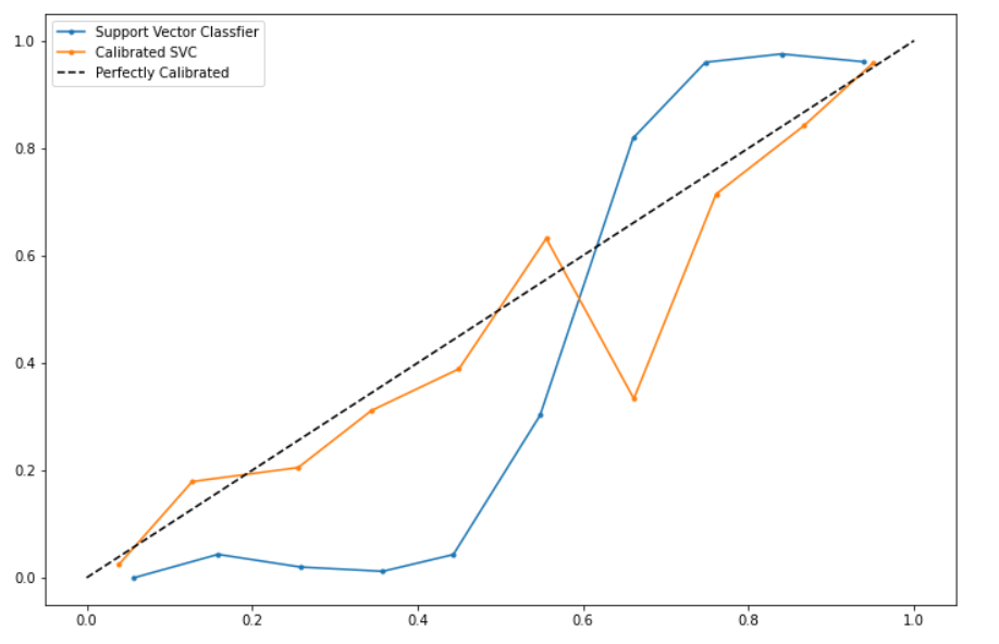
Well, generally Isotonic Regression is used in the probability calibration of classifiers. Probability Calibration of classifiers deals with the process of optimizing the output of classifiers so that the outputs of the classifier model can be directly interpreted as a confidence level. For example:- if the classifier classified that a certain number of samples belonged to a particular class with 90% probability then, roughly 90% of those samples should actually belong to that particular class.
There are mainly two ways of doing so:-
- Platt’s Scaling:- which fits a logistic regression model to the classifier model’s outputs.
- Isotonic Regression:- which fits an Isotonic or step like curve to the model’s outputs.
We will now see how Isotonic Regression is used in probability calibration:-
Note:- Although Isotonic Regression is more powerful than Platt Scaling in correcting monotonic distortions, it can easily overfit the data. The flexibility over Linear Regression comes with a price of more data requirement.
Let’s import the libraries:
from sklearn.datasets import make_classification
from sklearn.svm import SVC
from sklearn.calibration import CalibratedClassifierCV
from sklearn.model_selection import train_test_split
from sklearn.calibration import calibration_curve
Generating data and splitting it into train and test sets:
X, y = make_classification(n_samples=10000, n_classes=2, random_state=42)
trainX, testX, trainy, testy = train_test_split(X, y, test_size=0.2, random_state=42)
Fitting two models: One without calibration and one with calibration:
model1=SVC()
model1.fit(trainX,trainy)
preds1=model1.decision_function(testX)
model2=SVC()
cal=CalibratedClassifierCV(model2,method='isotonic',cv=5)
cal.fit(trainX,trainy)
preds2=cal.predict_proba(testX)[:,1]
Finding the calibration curves:
fop1, mpp1= calibration_curve(testy, preds1, n_bins=10, normalize=True)
fop2, mpp2= calibration_curve(testy, preds2, n_bins=10)
Plotting the curves:-
plt.figure(figsize=(12,8))
plt.plot(mpp1,fop1,marker='.')
plt.plot(mpp2,fop2,marker='.')
plt.plot([0,1],[0,1],linestyle='--',color='black')
plt.legend(("Support Vector Classfier","Calibrated SVC","Perfectly Calibrated"))
Result:
Conclusion
So now we know the basics of Isotonic Regression(believe me there’s more to this) and how it compares to Linear Regression. We also saw how it can be used in python and where to apply it. Finally, we got to know that the flexibility of Isotonic Regression in fitting monotonic functions better than Linear Regression comes at a price and that is more and more data.
I hope I was able to help anyone who wanted to learn the details of this algorithm at a deeper level. Also, I am thankful to everyone who gave this a read.
Due credits
The animation of the PAVA algorithm was borrowed from:-
https://www.r-bloggers.com/2020/05/what-is-isotonic-regression/
Follow these notes for more details:
http://www.stat.umn.edu/geyer/8054/notes/isotonic.pdf
Also, you can learn more about probability calibration from:-
https://machinelearningmastery.com/calibrated-classification-model-in-scikit-learn/
Credits for thumbnail image:-
https://realpython.com/linear-regression-in-python/#author
About me
I am a sophomore from Birla Institute Of Technology, Mesra, currently pursuing Electrical and Electronics Engineering. My interests lie in the fields of Machine Learning and Deep Learning and like robotics.
You can connect with me at:
You can also view some of the fun projects I worked on with my brother at:
https://www.youtube.com/channel/UC6J46NEyQEjag9fnOuBJ5hw
The media shown in this article are not owned by Analytics Vidhya and is used at the Author’s discretion.


