


Introduction
A popular and widely used statistical method for time series forecasting is the ARIMA model. Exponential smoothing and ARIMA models are the two most widely used approaches to time series forecasting and provide complementary approaches to the problem. While exponential smoothing models are based on a description of the trend and seasonality in the data, ARIMA models aim to describe the autocorrelations in the data. Before we talk about the ARIMA model, let’s talk about the concept of stationarity and the technique of differencing time series.
Table of contents
What is Autoregressive Integrated Moving Average (ARIMA)?
ARIMA is an acronym that stands for Auto-Regressive Integrated Moving Average. It is a class of model that captures a suite of different standard temporal structures in time series data.
In this tutorial, We will talk about how to develop an ARIMA model for time series forecasting in Python.
An ARIMA model is a class of statistical models for analyzing and forecasting time series data. It is really simplified in terms of using it, Yet this model is really powerful.
ARIMA stands for Auto-Regressive Integrated Moving Average.
The parameters of the ARIMA model are defined as follows:
- p: The number of lag observations included in the model, also called the lag order.
- d: The number of times that the raw observations are differenced, also called the degree of difference.
- q: The size of the moving average window, also called the order of moving average.
Steps to Use ARIMA Model
We construct a linear regression model by incorporating the specified number and type of terms. Additionally, we prepare the data through differencing to achieve stationarity, effectively eliminating trend and seasonal structures that can adversely impact the regression model.
- Visualize the Time Series Data
Visualize the Time Series Data involves plotting the historical data points over time to observe patterns, trends, and seasonality.
- Identify if the date is stationary
Identify if the data is stationary involves checking whether the time series data exhibits a stable pattern over time or if it has any trends or irregularities. Stationary data is necessary for accurate predictions using ARIMA, and various statistical tests can be employed to determine stationarity.
- Plot the Correlation and Auto Correlation Charts
To plot the correlation and auto-correlation charts in the steps of using the ARIMA model online, you analyze the time series data. The correlation chart displays the relationship between the current observation and lagged observations, while the auto-correlation chart shows the correlation of the time series with its own lagged values. These charts provide insights into potential patterns and dependencies within the data.
- Construct the ARIMA Model or Seasonal ARIMA based on the data
To construct an ARIMA (Autoregressive Integrated Moving Average) model or a Seasonal ARIMA model, one analyzes the data to determine the appropriate model parameters, such as the order of autoregressive (AR) and moving average (MA) components. This step involves selecting the optimal values for the model based on the characteristics and patterns observed in the data.
Stationarity
A stationary time series data is one whose properties do not depend on the time, That is why time series with trends, or with seasonality, are not stationary. the trend and seasonality will affect the value of the time series at different times, On the other hand for stationarity it does not matter when you observe it, it should look much the same at any point in time. In general, a stationary time series will have no predictable patterns in the long-term.
Let’s Start
import numpy as np
import pandas as pd
import matplotlib.pyplot as plt
%matplotlib inline
Defining the Dataset
In this tutorial, I am using the below dataset.
df=pd.read_csv('time_series_data.csv')
df.head()

# Updating the header
df.columns=["Month","Sales"]
df.head()
df.describe()
df.set_index('Month',inplace=True)

from pylab import rcParams
rcParams['figure.figsize'] = 15, 7
df.plot()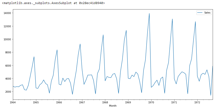
If we see the above graph then we will able to find a trend that there is a time when sales are high and vice versa. That means we can see data is following seasonality. For ARIMA first thing we do is identify if the data is stationary or non – stationary. if data is non-stationary we will try to make them stationary then we will process further.
Using Adfuller
Let’s check that if the given dataset is stationary or not, For that we use adfuller.
from statsmodels.tsa.stattools import adfullerI have imported the adfuller by running the above code.
test_result=adfuller(df['Sales'])To identify the nature of data, we will be using the null hypothesis.
- H0: The null hypothesis: It is a statement about the population that either is believed to be true or is used to put forth an argument unless it can be shown to be incorrect beyond a reasonable doubt.
- H1: The alternative hypothesis: It is a claim about the population that is contradictory to H0 and what we conclude when we reject H0.
#Ho: It is non-stationary
#H1: It is stationary
We will be considering the null hypothesis that data is not stationary and the alternate hypothesis that data is stationary.
def adfuller_test(sales):
    result=adfuller(sales)
    labels = ['ADF Test Statistic','p-value','#Lags Used','Number of Observations']
    for value,label in zip(result,labels):
        print(label+' : '+str(value) )

if result[1] <= 0.05:
    print("strong evidence against the null hypothesis(Ho), reject the null hypothesis. Data is stationary")
else:
    print("weak evidence against null hypothesis,indicating it is non-stationary ")

adfuller_test(df['Sales'])
Finding the P-value
After running the above code we will get P-value,
ADF Test Statistic : -1.8335930563276237
p-value : 0.3639157716602447
#Lags Used : 11
Number of Observations : 93
Here P-value is 0.36 which is greater than 0.05, which means data is accepting the null hypothesis, which means data is non-stationary.
Let’s try to see the first difference and seasonal difference:
df['Sales First Difference'] = df['Sales'] - df['Sales'].shift(1)
df['Seasonal First Difference']=df['Sales']-df['Sales'].shift(12)
df.head()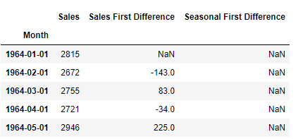
# Again testing if data is stationary
adfuller_test(df['Seasonal First Difference'].dropna())
ADF Test Statistic : -7.626619157213163
p-value : 2.060579696813685e-11
#Lags Used : 0
Number of Observations : 92Here P-value is 2.06, which means we will be rejecting the null hypothesis. So data is stationary.
df['Seasonal First Difference'].plot()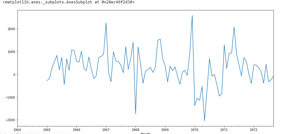
Create Auto-correlation
I am going to create auto-correlation :
from pandas.plotting import autocorrelation_plot
autocorrelation_plot(df['Sales'])
plt.show()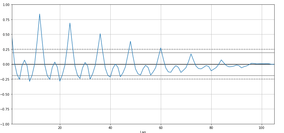
from statsmodels.graphics.tsaplots import plot_acf,plot_pacf
import statsmodels.api as sm
fig = plt.figure(figsize=(12,8))
ax1 = fig.add_subplot(211)
fig = sm.graphics.tsa.plot_acf(df['Seasonal First Difference'].dropna(),lags=40,ax=ax1)
ax2 = fig.add_subplot(212)
fig = sm.graphics.tsa.plot_pacf(df['Seasonal First Difference'].dropna(),lags=40,ax=ax2)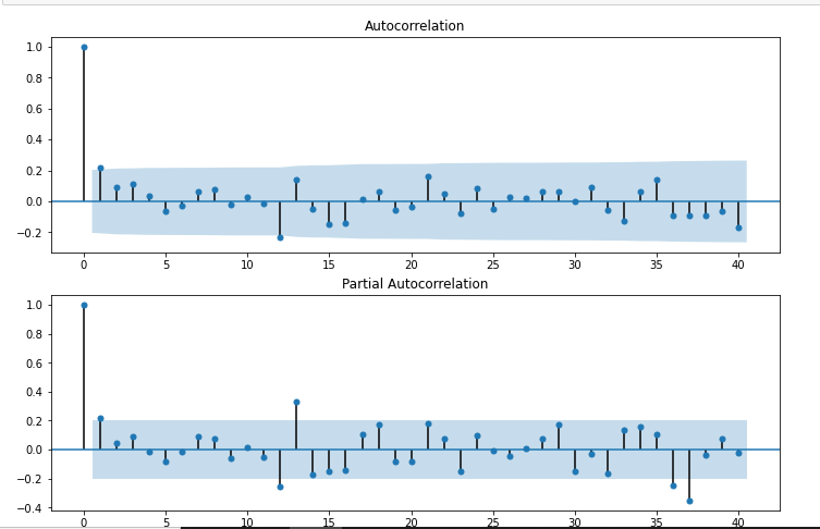
# For non-seasonal data
#p=1, d=1, q=0 or 1

from statsmodels.tsa.arima_model import ARIMA
model=ARIMA(df['Sales'],order=(1,1,1))
model_fit=model.fit()
model_fit.summary()| Dep. Variable: | D.Sales | No. Observations: | 104 |
|---|---|---|---|
| Model: | ARIMA(1, 1, 1) | Log-Likelihood | -951.126 |
| Method: | css-mle | S.D. of innovations | 2227.262 |
| Date: | Wed, 28 Oct 2020 | AIC | 1910.251 |
| Time: | 11:49:08 | BIC | 1920.829 |
| Sample: | 02-01-1964 to 09-01-1972 | HQIC | 1914.536 |
| coef | std err | z | P>|z| | [0.025 | 0.975] | |
|---|---|---|---|---|---|---|
| const | 22.7845 | 12.405 | 1.837 | 0.066 | -1.529 | 47.098 |
| ar.L1.D.Sales | 0.4343 | 0.089 | 4.866 | 0.000 | 0.259 | 0.609 |
| ma.L1.D.Sales | -1.0000 | 0.026 | -38.503 | 0.000 | -1.051 | -0.949 |
| Real | Imaginary | Modulus | Frequency | |
|---|---|---|---|---|
| AR.1 | 2.3023 | +0.0000j | 2.3023 | 0.0000 |
| MA.1 | 1.0000 | +0.0000j | 1.0000 | 0.0000 |
df['forecast']=model_fit.predict(start=90,end=103,dynamic=True)
df[['Sales','forecast']].plot(figsize=(12,8))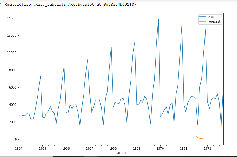
import statsmodels.api as sm
model=sm.tsa.statespace.SARIMAX(df['Sales'],order=(1, 1, 1),seasonal_order=(1,1,1,12))
results=model.fit()
df['forecast']=results.predict(start=90,end=103,dynamic=True)
df[['Sales','forecast']].plot(figsize=(12,8))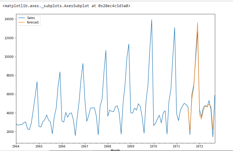
from pandas.tseries.offsets import DateOffset
future_dates=[df.index[-1]+ DateOffset(months=x)for x in range(0,24)]
future_datest_df=pd.DataFrame(index=future_dates[1:],columns=df.columns)

future_datest_df.tail()

future_df=pd.concat([df,future_datest_df])

future_df['forecast'] = results.predict(start = 104, end = 120, dynamic= True)
future_df[['Sales', 'forecast']].plot(figsize=(12, 8))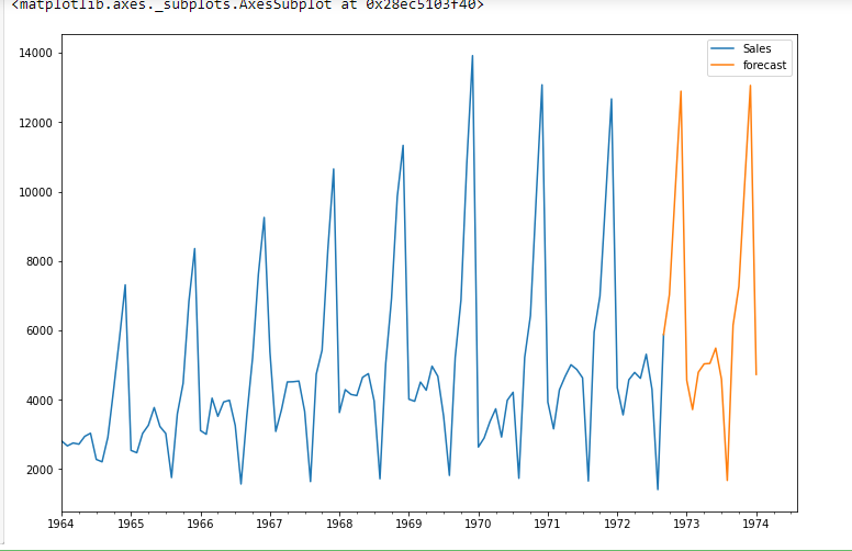
Conclusion
Time Series forecasting is really useful when we have to take future decisions or we have to do analysis, we can quickly do that using ARIMA, there are lots of other Models from we can do the time series forecasting but ARIMA model is really easy to understand. If you’re interested in mastering data science techniques like ARIMA, explore enrolling in the renowned Blackbelt Plus Program. This step will enhance your skills and broaden your horizons in this dynamic field, marking the beginning of your data science journey today!
Frequently Asked Questions
A. ARIMA, or AutoRegressive Integrated Moving Average, is a time series forecasting method implemented in Python for predicting future data points based on historical time series data.
A. ARIMA and regression serve different purposes. ARIMA is suitable for time series data, while regression is used for modeling relationships between variables. The choice depends on the data and the problem.
A. No, ARIMA and regression are different. ARIMA is designed for time series forecasting, focusing on temporal patterns, while regression models the relationship between variables, irrespective of time.
A. ARIMA is a powerful technique for time series forecasting. It models time-dependent patterns, such as trends and seasonality, making it valuable for predicting future values in sequential data.