This article was published as a part of the Data Science Blogathon.
Overview
- This article is a continuation and Part 2 of my first blog article on Analytics Vidhya – Ultimate Beginners Guide to Breaking into the Top 10% in Machine Learning Hackathons
- Winning Classification Hackathons is an easy process if you follow these simple steps listed in this article
- Always keep learning continuously, experiment with great consistency, and follow your intuition and domain knowledge that you build over time
- From a beginner in Hackathons a few months back, I have recently become a Kaggle Expert and one of the TOP 5 Contributors of Analytics Vidhya’s JanataHack Hackathon Series
- I am here to share my knowledge and guide beginners to Top Hackathons with Classification Use Cases in Binary Classification
Source : https://unsplash.com/photos/KI0_WS7OrmA
Let’s Deep Dive into the Binary Classification – Insurance Cross-Sell Use Case from Analytics Vidhya’s JanataHack Hackathon Series and get our hands dirty
Our client is an Insurance company that has provided Health Insurance to its customers. Now they need our help in building a model to predict whether the policyholders (customers) from the past year will also be interested in Vehicle Insurance provided by the company.
An insurance policy is an arrangement by which a company undertakes to provide a guarantee of compensation for specified loss, damage, illness, or death in return for the payment of a specified premium. A premium is a sum of money that the customer needs to pay regularly to an insurance company for this guarantee.
For example, we may pay a premium of Rs. 5000 each year for a health insurance cover of Rs. 200,000/- so that if God forbid, we fall ill and need to be hospitalized in that year, the insurance provider company will bear the cost of hospitalization, etc. for up to Rs. 200,000. Now if we are wondering how can the company bear such high hospitalization costs when it charges a premium of only Rs. 5000/-, that is where the concept of probabilities comes into the picture.
For example, like us, there may be 100 customers who would be paying a premium of Rs. 5000 every year, but only a few of them (say 2-3) would get hospitalized that year. This way everyone shares the risk of everyone else.
Just like medical insurance, there is vehicle insurance where every year customer needs to pay a premium of a certain amount to the insurance provider company so that in case of an unfortunate accident by the vehicle, the insurance provider company will provide a compensation (called ‘sum assured’) to the customer.
Building a model to predict whether a customer would be interested in Vehicle Insurance is extremely helpful for the company because it can then accordingly plan its communication strategy to reach out to those customers and optimize its business model and revenue.
Sharing my Data Science Hackathon Approach – How to reach Top 10% among 20,000+ Data Lovers
In Part 1, we learned a 10 Step Process that can be repeated, optimized, and improved, which is a great foundation to help you get started quickly.
Now that you would have started practicing, let us try our hand on an Insurance Use Case to test our skills. Rest assured, you will be in a good position to tackle any Classification Hackathons (with table data) with a few weeks of practice. Hope you are enthusiastic, curious to learn, and excited to continue this Data Science journey with Hackathons!
10 Easy Steps to Learn, Practice and Top in Classification Hackathons
- Understand the Problem Statement and Import the Packages and Datasets
- Perform EDA (Exploratory Data Analysis) – Understanding the Datasets. Explore Train and Test Data and get to know what each Column / Feature denotes. Check for Imbalance of Target Column in Datasets
- Check for Duplicate Rows from Train Data
- Fill/Impute Missing Values – Continuous – Mean/Median/Any Specific Value | Categorical – Others/ForwardFill/BackFill
- Feature Engineering – Feature Selection – Selection of Most Important Existing Features | Feature Creation or Binning – Creation of New Feature(s) from the Existing Feature(s)
- Split Train Data into Features(Independent Variables) | Target(Dependent Variable)
- Data Encoding – Label Encoding, One-Hot Encoding | Data Scaling – MinMaxScaler, StandardScaler, RobustScaler
- Create Baseline Machine Learning Model for the Binary Classification problem
- Ensemble with Averaging to Improve the Evaluation Metric “ROC_AUC” with K-FOLD CROSS VALIDATION and Predict Target “Response”
- Result Submission, Check Leaderboard and Improve “ROC_AUC”
1. Understand the Problem Statement and Import Packages and Datasets
Dataset Description
| Variable | Definition |
| id | Unique ID for the customer |
| Gender | Gender of the customer |
| Age | Age of the customer |
| Driving_License | 0 : Customer does not have DL, 1 : Customer already has DL |
| Region_Code | Unique code for the region of the customer |
| Previously_Insured | 1 : Customer already has Vehicle Insurance, 0 : Customer doesn’t have Vehicle Insurance |
| Vehicle_Age | Age of the Vehicle |
| Vehicle_Damage | 1 : Customer got his/her vehicle damaged in the past. |
| 0 : Customer didn’t get his/her vehicle damaged in the past. | |
| Annual_Premium | The amount customer needs to pay as premium in the year |
| Policy_Sales_Channel | Anonymised Code for the channel of outreaching to the customer ie. Different Agents, Over Mail, Over Phone, In Person, etc. |
| Vintage | Number of Days, Customer has been associated with the company |
| Response | 1 : Customer is interested, 0 : Customer is not interested |
Now, in order to predict whether the customer would be interested in Vehicle insurance, we have information about Demographics (gender, age, region code type), Vehicles (Vehicle Age, Damage), Policy (Premium, sourcing channel), etc.
Evaluation Metric used to Check Machine Learning Models Performance Differs in All Hackathons
Here we have ROC_AUC as the Evaluation Metric.
The Receiver Operator Characteristic (ROC) curve is an evaluation metric for binary classification problems. It is a probability curve that plots the TPR (True Positive Rate) against FPR (False Positive Rate) at various threshold values and essentially separates the ‘signal’ from the ‘noise’. The Area Under the Curve (AUC) is the measure of the ability of a classifier to distinguish between classes and is used as a summary of the ROC curve.
The higher the AUC, the better the performance of the model at distinguishing between the positive and negative classes.
- When AUC = 1 the classifier is able to perfectly distinguish between all the Positive and the Negative class points correctly. If, however, the AUC had been 0, then the classifier would be predicting all Negatives as Positives, and all Positives as Negatives.
- When 0.5<AUC<1 there is a high chance that the classifier will be able to distinguish the positive class values from the negative class values. This is so because the classifier is able to detect more numbers of True positives and True negatives than False negatives and False positives.
- When AUC=0.5 then the classifier is not able to distinguish between Positive and Negative class points. Meaning either the classifier is predicting random class or constant class for all the data points.
- Cross-Sell: Train Data consists of 3,81,109 examples, and the Test Data consists of 1,27,037 examples. Huge Imbalance in Data again – only 12.25% (46,709 out of a total 3,81,109) of Employees were recommended for promotion based on Train data.
Let us start by Importing the required Python Packages
# Import Required Python Packages
# Scientific and Data Manipulation Libraries
import numpy as np
import pandas as pd

# Data Viz & Regular Expression Libraries
import matplotlib.pyplot as plt
import seaborn as sns

# Scikit-Learn Pre-Processing Libraries
from sklearn.preprocessing import *

# Garbage Collection Libraries
import gc

# Boosting Algorithm Libraries
from xgboost import XGBClassifier
from catboost import CatBoostClassifier
from lightgbm import LGBMClassifier

# Model Evaluation Metric & Cross Validation Libraries
from sklearn.metrics import roc_auc_score, auc, roc_curve
from sklearn.model_selection import StratifiedKFold, KFold

# Setting SEED to Reproduce Same Results even with "GPU"
seed_value = 1994
import os
os.environ['PYTHONHASHSEED'} = str(seed_value)
import random
random.seed(seed_value)
import numpy as np
np.random.seed(seed_value)
SEED=seed_value
- Scientific and Data Manipulation – Used to manipulate Numeric data using Numpy and Table data using Pandas.
- Data Visualization Libraries – Matplotlib and Seaborn are used for visualization of the single or multiple variables.
- Data Preprocessing, Machine Learning, and Metrics Libraries – Used to pre-process the data by encoding, scaling, and measure the date using evaluating metrics like ROC_AUC Score.
- Boosting Algorithms – XGBoost, CatBoost, and LightGBM Tree-based Classifier Models are used for Binary as well as Multi-Class classification
- Setting SEED – Used to set the SEED to Reproduce the Same Results every time
2. Perform EDA (Exploratory Data Analysis) – Understanding the Datasets
Python Code:
# Python Method 1 : Displays Data Information
def display_data_information(data, data_types, df)
data.info()
print("\n")
for VARIABLE in data_types :
data_type = data.select_dtypes(include=[ VARIABLE }).dtypes
if len(data_type) > 0 :
print(str(len(data_type))+" "+VARIABLE+" Features\n"+str(data_type)+"\n" )

# Display Data Information of "train" :
data_types = ["float32","float64","int32","int64","object","category","datetime64[ns}"}
display_data_information(train, data_types, "train")

# Display Data Information of "test" :
display_data_information(test, data_types, "test")

# Python Method 2 : Displays Data Head (Top Rows) and Tail (Bottom Rows) of the Dataframe (Table) :
def display_head_tail(data, head_rows, tail_rows)
display("Data Head & Tail :")
display(data.head(head_rows).append(data.tail(tail_rows)))

#     return True
# Displays Data Head (Top Rows) and Tail (Bottom Rows) of the Dataframe (Table)
# Pass Dataframe as "train", No. of Rows in Head = 3 and No. of Rows in Tail = 2 :
display_head_tail(train, head_rows=3, tail_rows=2)

# Python Method 3 : Displays Data Description using Statistics :
def display_data_description(data, numeric_data_types, categorical_data_types)
print("Data Description :")
display(data.describe( include = numeric_data_types))
print("")
display(data.describe( include = categorical_data_types))

# Display Data Description of "train" :
display_data_description(train, data_types[0:4}, data_types[4:7})

# Display Data Description of "test" :
display_data_description(test, data_types[0:4}, data_types[4:7})
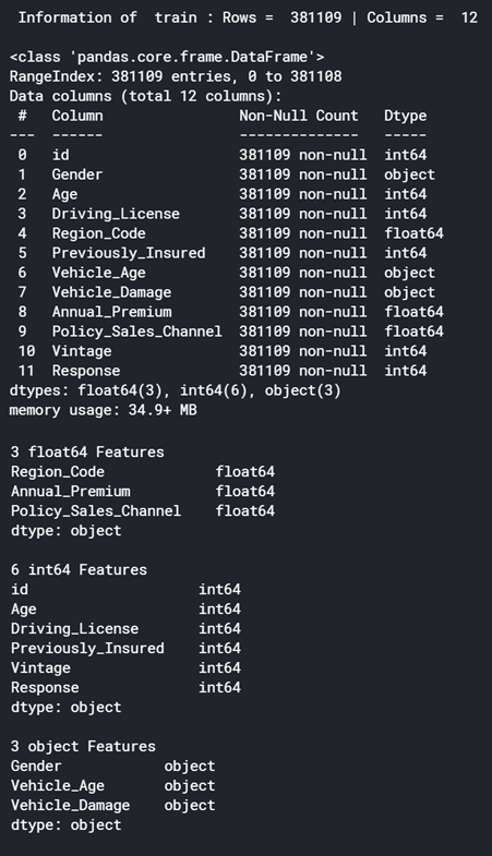
Reading the Data Files in CSV Format – Pandas read_csv method is used to read the csv file and convert into a Table like Data structure called a DataFrame. So 3 DataFrames are created for Train, Test and Submission.
Apply Head and Tail on Data – Used to view the Top 3 rows and Last 2 rows to get an overview of the data.
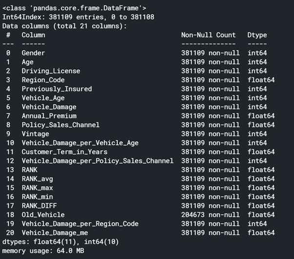
Apply Info on Data – Used to display information on Columns, Data Types and Memory usage of the DataFrames.
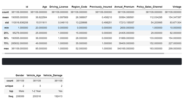
Apply Describe on Data – Used to display the Descriptive statistics like Count, Unique, Mean, Min, Max .etc on Numerical Columns.
3. Check for Duplicate Rows from Train Data
# Removes Data Duplicates while Retaining the First one
def remove_duplicate(data)
data.drop_duplicates(keep="first", inplace=True)
return "Checked Duplicates
# Removes Duplicates from train data
remove_duplicate(train)
Checking the Train Data for Duplicates – Removes the duplicate rows by keeping the first row. No duplicates were found in Train data.
4. Fill/Impute Missing Values – Continuous – Mean/Median/Zero(Specific Value) | Categorical – Forward/BackFill/Others
There are no missing values in the data.
5. Feature Engineering
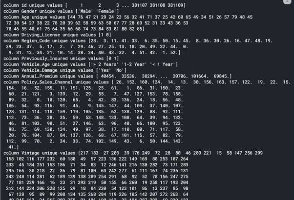
# Check train data for Values of each Column - Short Form
for i in train
print(f'column {i} unique values {train[i}.unique()})
# Binary Classification Problem - Target has ONLY 2 Categories
# Target - Response has 2 Values of Customers 1 & 0
# Combine train and test data into single DataFrame - combine_set
combine_set = pd.concat{[train,test},axis=0}
# converting object to int type :
combine_set['Vehicle_Age'}=combine_set['Vehicle_Age'}.replacee({'< 1 Year':0,'1-2 Year':1,'> 2 Years':2})
combine_set['Gender'}=combine_set['Gender'}.replacee({'Male':1,'Female':0})
combine_set['Vehicle_Damage'}=combine_set['Vehicle_Damage'}.replacee({'Yes':1,'No':0})
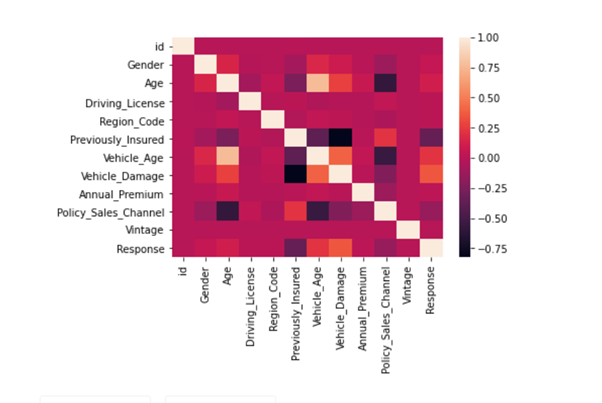
sns.heatmap(combine_set.corr())
# HOLD - CV - 0.8589 - BEST EVER
combine_set['Vehicle_Damage_per_Vehicle_Age'} = combine_set.groupby(['Region_Code,Age'})['Vehicle_Damage'}.transform('sum'
# Score - 0.858657 (This Feature + Removed Scale_Pos_weight in LGBM) | Rank - 20
combine_set['Customer_Term_in_Years'} = combine_set['Vintage'} / 365
# combine_set['Customer_Term'} = (combine_set['Vintage'} / 365).astype('str')
# Score - 0.85855 | Rank - 20
combine_set['Vehicle_Damage_per_Policy_Sales_Channel'} = combine_set.groupby(['Region_Code,Policy_Sales_Channel'})['Vehicle_Damage'}.transform('sum')
# Score - 0.858527 | Rank - 22
combine_set['Vehicle_Damage_per_Vehicle_Age'} = combine_set.groupby(['Region_Code,Vehicle_Age'})['Vehicle_Damage'}.transform('sum')
# Score - 0.858510 | Rank - 23
combine_set["RANK"} = combine_set.groupby("id")['id'}.rank(method="first", ascending=True)
combine_set["RANK_avg"} = combine_set.groupby("id")['id'}.rank(method="average", ascending=True)
combine_set["RANK_max"} = combine_set.groupby("id")['id'}.rank(method="max", ascending=True)
combine_set["RANK_min"} = combine_set.groupby("id")['id'}.rank(method="min", ascending=True)
combine_set["RANK_DIFF"} = combine_set['RANK_max'} - combine_set['RANK_min'}
# Score - 0.85838 | Rank - 15
combine_set['Vehicle_Damage_per_Vehicle_Age'} = combine_set.groupby([Region_Code})['Vehicle_Damage'}.transform('sum')

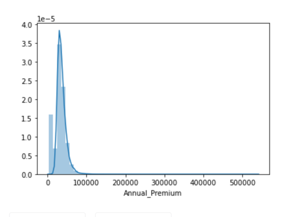
# Data is left Skewed as we can see from below distplot
sns.distplot(combine_set['Annual_Premium'})
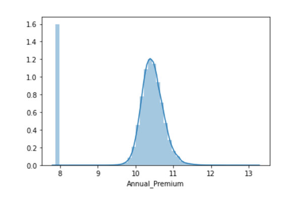
combine_set['Annual_Premium'} = np.log(combine_set['Annual_Premium'})
sns.distplot(combine_set['Annual_Premium'})
# Getting back Train and Test after Preprocessing :
train=combine_set[combine_set['Response'}.isnull()==False}
test=combine_set[combine_set['Response'}.isnull()==True}.drop(['Response'},axis=1)
train.columns
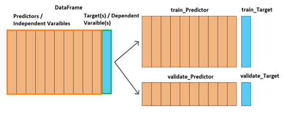
6. Split Train Data into Train and Validation Data with Predictors (Independent) & Target (Dependent)
# Split the Train data into predictors and target :
predictor_train = train.drop(['Response','id'],axis=1)
target_train    = train['Response']
predictor_train.head()
# Get the Test data by dropping 'id' :
predictor_test = test.drop(['id'],axis=1)
7. Data Encoding – Target Encoding
def add_noise(series, noise_level):
return series * (1 + noise_level * np.random.randn(len(series)))
def target_encode(trn_series=None,
tst_series=None,
target=None,
min_samples_leaf=1,
smoothing=1,
noise_level=0):
"""
Smoothing is computed like in the following paper by Daniele Micci-Barreca
https://kaggle2.blob.core.windows.net/forum-message-attachments/225952/7441/high%20cardinality%20categoricals.pdf

trn_series : training categorical feature as a pd.Series
tst_series : test categorical feature as a pd.Series
target : target data as a pd.Series
min_samples_leaf (int) : minimum samples to take category average into account
smoothing (int) : smoothing effect to balance categorical average vs prior
"""
assert len(trn_series) == len(target)
assert trn_series.name == tst_series.name
temp = pd.concat([trn_series, target], axis=1)
# Compute target mean
averages = temp.groupby(by=trn_series.name)[target.name].agg(["mean", "count"])
# Compute smoothing
smoothing = 1 / (1 + np.exp(-(averages["count"] - min_samples_leaf) / smoothing))
# Apply average function to all target data
prior = target.mean()
# The bigger the count the less full_avg is taken into account
averages[target.name] = prior * (1 - smoothing) + averages["mean"] * smoothing
averages.drop(["mean", "count"], axis=1, inplace=True)
# Apply averages to trn and tst series
ft_trn_series = pd.merge(
trn_series.to_frame(trn_series.name),
averages.reset_index().rename(columns={'index': target.name, target.name: 'average'}),
on=trn_series.name,
how='left')['average'].rename(trn_series.name + '_mean').fillna(prior)
# pd.merge does not keep the index so restore it
ft_trn_series.index = trn_series.index
ft_tst_series = pd.merge(
tst_series.to_frame(tst_series.name),
averages.reset_index().rename(columns={'index': target.name, target.name: 'average'}),
on=tst_series.name,
how='left')['average'].rename(trn_series.name + '_mean').fillna(prior)
# pd.merge does not keep the index so restore it
ft_tst_series.index = tst_series.index
return add_noise(ft_trn_series, noise_level), add_noise(ft_tst_series, noise_level)
# Score - 0.85857 | Rank -
tr_g, te_g = target_encode(predictor_train["Vehicle_Damage"],
predictor_test["Vehicle_Damage"],
target= predictor_train["Response"],
min_samples_leaf=200,
smoothing=20,
noise_level=0.02)
predictor_train['Vehicle_Damage_me']=tr_g
predictor_test['Vehicle_Damage_me']=te_g
8. Create Baseline Machine Learning Model for Binary Classification Problem
# Baseline Model Without Hyperparameters :
Classifiers = {'0.XGBoost' : XGBClassifier(),
'1.CatBoost' : CatBoostClassifier(),
'2.LightGBM' : LGBMClassifier()
}
# Fine Tuned Model With-Hyperparameters :
Classifiers = {'0.XGBoost' : XGBClassifier(eval_metric='auc',

# GPU PARAMETERS #
tree_method='gpu_hist',
gpu_id=0,

# GPU PARAMETERS #
random_state=294,
learning_rate=0.15,
max_depth=4,
n_estimators=494,
objective='binary:logistic'),
'1.CatBoost' : CatBoostClassifier(eval_metric='AUC',

# GPU PARAMETERS #
task_type='GPU',
devices="0",

# GPU PARAMETERS #
learning_rate=0.15,
n_estimators=494,
max_depth=7,
#                             scale_pos_weight=2),

'2.LightGBM' : LGBMClassifier(metric = 'auc',

# GPU PARAMETERS #
device = "gpu",
gpu_device_id =0,
max_bin = 63,
gpu_platform_id=1,

# GPU PARAMETERS #
n_estimators=50000,
bagging_fraction=0.95,
subsample_freq = 2,
objective ="binary",
min_samples_leaf= 2,
importance_type = "gain",
verbosity = -1,
random_state=294,
num_leaves = 300,
boosting_type = 'gbdt',
learning_rate=0.15,
max_depth=4,

# scale_pos_weight=2, # Score - 0.85865 | Rank - 18
n_jobs=-1)
}
9. Ensemble with Averaging to Improve the Evaluation Metric “ROC_AUC” with K-FOLD CROSS VALIDATION and Predict Target “Response”
# LightGBM Model
kf=KFold(n_splits=10,shuffle=True)
preds_1   = list()
y_pred_1  = []
rocauc_score = []
for i,(train_idx,val_idx) in enumerate(kf.split(predictor_train)):
X_train, y_train = predictor_train.iloc[train_idx,:], target_train.iloc[train_idx]
X_val, y_val = predictor_train.iloc[val_idx, :], target_train.iloc[val_idx]
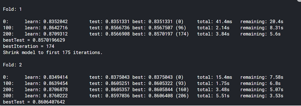
print('\nFold: {}\n'.format(i+1))
lg= LGBMClassifier(      metric = 'auc',

# GPU PARAMETERS #
device = "gpu",
gpu_device_id =0,
max_bin = 63,
gpu_platform_id=1,

# GPU PARAMETERS #
n_estimators=50000,
bagging_fraction=0.95,
subsample_freq = 2,
objective ="binary",
min_samples_leaf= 2,
importance_type = "gain",
verbosity = -1,
random_state=294,
num_leaves = 300,
boosting_type = 'gbdt',
learning_rate=0.15,
max_depth=4,
# scale_pos_weight=2, # Score - 0.85865 | Rank - 18
n_jobs=-1
)
lg.fit(X_train, y_train
,eval_set=[(X_train, y_train),(X_val, y_val)]
,early_stopping_rounds=100
,verbose=100
)
roc_auc = roc_auc_score(y_val,lg.predict_proba(X_val)[:, 1])
rocauc_score.append(roc_auc)
preds_1.append(lg.predict_proba(predictor_test [predictor_test.columns])[:, 1])
y_pred_final_1          = np.mean(preds_1,axis=0)
sub['Response']=y_pred_final_1
Blend_model_1 = sub.copy()
print('ROC_AUC - CV Score: {}'.format((sum(rocauc_score)/10)),'\n')
print("Score : ",rocauc_score)
# Download and Show Submission File :
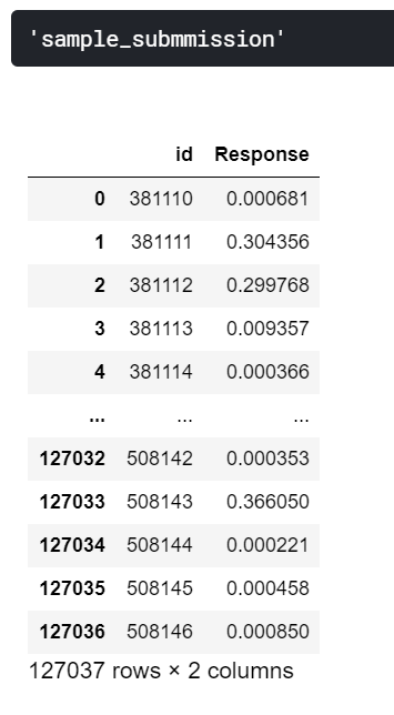
display("sample_submmission",sub)
sub_file_name_1 = "S1. LGBM_GPU_TargetEnc_Vehicle_Damage_me_1994SEED_NoScaler.csv"
sub.to_csv(sub_file_name_1,index=False)
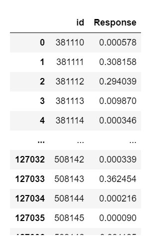
sub.head(5)
# Catboost Model
kf=KFold(n_splits=10,shuffle=True)
preds_2   = list()
y_pred_2  = []
rocauc_score = []
for i,(train_idx,val_idx) in enumerate(kf.split(predictor_train)):
X_train, y_train = predictor_train.iloc[train_idx,:], target_train.iloc[train_idx]
X_val, y_val = predictor_train.iloc[val_idx, :], target_train.iloc[val_idx]
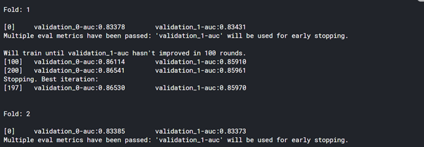
print('\nFold: {}\n'.format(i+1))
cb = CatBoostClassifier( eval_metric='AUC',

# GPU PARAMETERS #
task_type='GPU',
devices="0",

# GPU PARAMETERS #
learning_rate=0.15,
n_estimators=494,
max_depth=7,
#                             scale_pos_weight=2
)
cb.fit(X_train, y_train
,eval_set=[(X_val, y_val)]
,early_stopping_rounds=100
,verbose=100
)
roc_auc = roc_auc_score(y_val,cb.predict_proba(X_val)[:, 1])
rocauc_score.append(roc_auc)
preds_2.append(cb.predict_proba(predictor_test [predictor_test.columns])[:, 1])
y_pred_final_2          = np.mean(preds_2,axis=0)
sub['Response']=y_pred_final_2
print('ROC_AUC - CV Score: {}'.format((sum(rocauc_score)/10)),'\n')
print("Score : ",rocauc_score)
# Download and Show Submission File :
display("sample_submmission",sub)
sub_file_name_2 = "S2. CB_GPU_TargetEnc_Vehicle_Damage_me_1994SEED_LGBM_NoScaler_MyStyle.csv"
sub.to_csv(sub_file_name_2,index=False)
Blend_model_2 = sub.copy()
sub.head(5)
# XGBOOST Model
kf=KFold(n_splits=10,shuffle=True)
preds_3   = list()
y_pred_3  = []
rocauc_score = []
for i,(train_idx,val_idx) in enumerate(kf.split(predictor_train)):
X_train, y_train = predictor_train.iloc[train_idx,:], target_train.iloc[train_idx]
X_val, y_val = predictor_train.iloc[val_idx, :], target_train.iloc[val_idx]
print('\nFold: {}\n'.format(i+1))
xg=XGBClassifier( eval_metric='auc',

# GPU PARAMETERS #
tree_method='gpu_hist',
gpu_id=0,

# GPU PARAMETERS #
random_state=294,
learning_rate=0.15,
max_depth=4,
n_estimators=494,
objective='binary:logistic'
)
xg.fit(X_train, y_train
,eval_set=[(X_train, y_train),(X_val, y_val)]
,early_stopping_rounds=100
,verbose=100
)
roc_auc = roc_auc_score(y_val,xg.predict_proba(X_val)[:, 1])
rocauc_score.append(roc_auc)
preds_3.append(xg.predict_proba(predictor_test [predictor_test.columns])[:, 1])
y_pred_final_3         = np.mean(preds_3,axis=0)
sub['Response']=y_pred_final_3
print('ROC_AUC - CV Score: {}'.format((sum(rocauc_score)/10)),'\n')
print("Score : ",rocauc_score)
# Download and Show Submission File :
display("sample_submmission",sub)
sub_file_name_3 = "S3. XGB_GPU_TargetEnc_Vehicle_Damage_me_1994SEED_LGBM_NoScaler.csv"
sub.to_csv(sub_file_name_3,index=False)
Blend_model_3 = sub.copy()
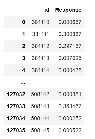
sub.head(5)
10. Result Submission, Check Leaderboard & Improve “ROC_AUC” Score
one = Blend_model_2['id'].copy()
Blend_model_1.drop("id", axis=1, inplace=True)
Blend_model_2.drop("id", axis=1, inplace=True)
Blend_model_3.drop("id", axis=1, inplace=True)
Blend = (Blend_model_1 + Blend_model_2 + Blend_model_3)/3
id_df = pd.DataFrame(one, columns=['id'])
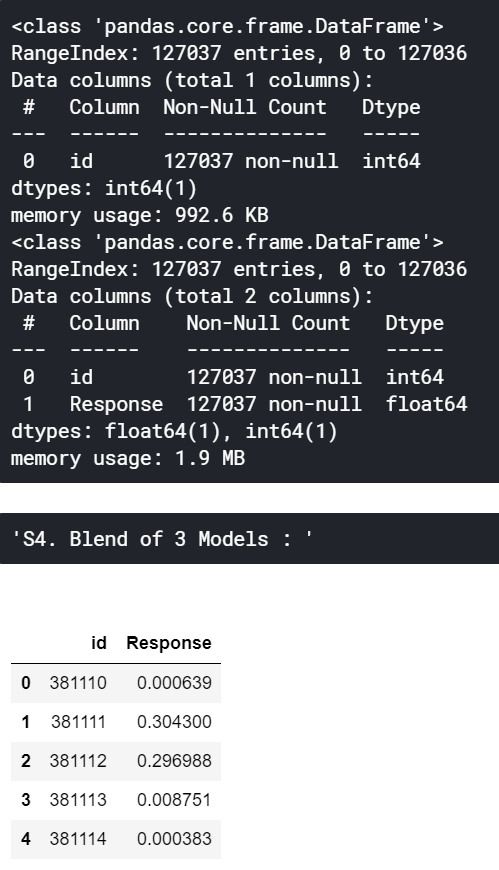
id_df.info()
Blend = pd.concat([ id_df,Blend], axis=1)
Blend.info()
Blend.to_csv('S4. Blend of 3 Models - LGBM_CB_XGB.csv',index=False)
display("S4. Blend of 3 Models : ",Blend.head())
k-Fold Cross-Validation
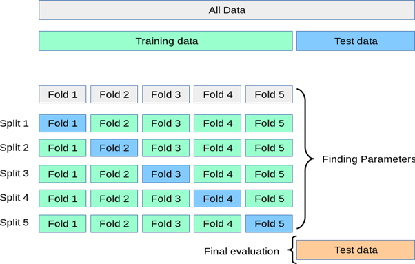
Cross-validation is a resampling procedure used to evaluate machine learning models on a limited data sample. The procedure has a single parameter called k that refers to the number of groups that a given data sample is to be split into. As such, the procedure is often called k-fold cross-validation.
Example of k-Fold k=5, 5-Fold Cross-Validation.
Source: Scikit Learn Documentation – https://scikit-learn.org/stable/modules/cross_validation.html
Early Stopping Rounds
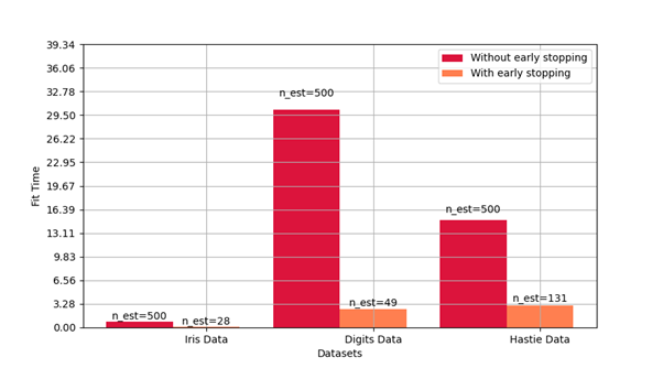
- In machine learning, early stopping is a form of regularization used to avoid overfitting when training a learner with an iterative method, such as gradient descent.
- Early stopping rules provide guidance as to how many iterations can be run before the learner begins to over-fit.
- Documentation here
How to Make all 3 Machine Learning Models on GPU run Faster
1. GPU PARAMETERS in LIGHTGBM
To use LightGBM GPU Model : “Internet” need to be on – Run all the code Below :
# Keep Internet “On” which is present in right side -> Settings Panel in Kaggle Kernel
# Cell 1 :
!rm -r /opt/conda/lib/python3.6/site-packages/lightgbm
!git clone –recursive https://github.com/Microsoft/LightGBM
# Cell 2 :
!apt-get install -y -qq libboost-all-dev
# Cell 3 :
%%bash
cd LightGBM
rm -r build
mkdir build
cd build
cmake -DUSE_GPU=1 -DOpenCL_LIBRARY=/usr/local/cuda/lib64/libOpenCL.so -DOpenCL_INCLUDE_DIR=/usr/local/cuda/include/ ..
make -j$(nproc)
# Cell 4 :
!cd LightGBM/python-package/;python3 setup.py install –precompile
# Cell 5 :
!mkdir -p /etc/OpenCL/vendors && echo “libnvidia-opencl.so.1” > /etc/OpenCL/vendors/nvidia.icd
!rm -r LightGBM
- device = “gpu”
- gpu_device_id =0
- max_bin = 63
- gpu_platform_id=1
How to Achieve Good Speed on GPU
- You want to run a few datasets that we have verified with good speedup (including Higgs, epsilon, Bosch, etc) to ensure your setup is correct. If you have multiple GPUs, make sure to set gpu_platform_id and gpu_device_id to use the desired GPU. Also make sure your system is idle (especially when using a shared computer) to get accuracy performance measurements.
- GPU works best on large scale and dense datasets. If dataset is too small, computing it on GPU is inefficient as the data transfer overhead can be significant. If you have categorical features, use the categorical_column option and input them into LightGBM directly; do not convert them into one-hot variables.
- To get good speedup with GPU, it is suggested to use a smaller number of bins. Setting max_bin=63 is recommended, as it usually does not noticeably affect training accuracy on large datasets, but GPU training can be significantly faster than using the default bin size of 255. For some dataset, even using 15 bins is enough (max_bin=15); using 15 bins will maximize GPU performance. Make sure to check the run log and verify that the desired number of bins is used.
- Try to use single-precision training (gpu_use_dp=false) when possible, because most GPUs (especially NVIDIA consumer GPUs) have poor double-precision performance.
2. GPU PARAMETERS in CATBOOST
- task_type=’GPU’
- devices=”0″
| Parameters | Description | |
| · CatBoost (fit)
· CatBoostRegressor (fit) |
task_type | The processing unit type to use for training.
Possible values: · CPU · GPU |
| devices | IDs of the GPU devices to use for training (indices are zero-based).
Format · <unit ID> for one device (for example, 3) · <unit ID1>:<unit ID2>:..:<unit IDN> for multiple devices (for example, devices=’0:1:3′) · <unit ID1>-<unit IDN> for a range of devices (for example, devices=’0-3′) |
3. GPU PARAMETERS in XGBOOST
- tree_method=’gpu_hist’
- gpu_id=0
Usage
Specify the tree_method parameter as one of the following algorithms.
Algorithms
| tree_method | Description |
| gpu_hist | Equivalent to the XGBoost fast histogram algorithm. Much faster and uses considerably less memory. NOTE: May run very slowly on GPUs older than Pascal architecture. |
Supported parameters
| parameter | gpu_hist |
| subsample | ✔ |
| sampling_method | ✔ |
| colsample_bytree | ✔ |
| colsample_bylevel | ✔ |
| max_bin | ✔ |
| gamma | ✔ |
| gpu_id | ✔ |
| predictor | ✔ |
| grow_policy | ✔ |
| monotone_constraints | ✔ |
| interaction_constraints | ✔ |
| single_precision_histogram | ✔ |
Summary of the Cross-Sell Hackathon
“10” Things that Worked in this AV Cross-Sell Hackathon:
- 2 BEST Features – Target Encoding of Vehicle_Damage and Sum of Vehicle_Damage Grouped by Region_Code – Based on Feature Importance – Gave a Good Boost in CV(10-Fold Cross Validation) and LB(Public LeaderBoard).
- Domain-Based Feature: Frequency Encoding of Old Vehicle – Gave a little Boost. LB Score – 0.85838 | LB Rank – 15
- Rank Features from Hackathon Solutions – Gave a Huge Boost. LB Score – 0.858510 | LB Rank – 23
- Dropping “id” Column – Gave a Good Boost.
- Domain-Based Feature: Vehicle_Damage per Vehicle_Age & Region_Code – Gave a little Boost. LB Score – 0.858527 | LB Rank – 22
- Removing Skew in Annual_Premium – Gave a Huge Boost. Score – 0.85857 LB Score – 0.85855 | LB Rank – 20
- Domain Based Feature: Vehicle_Damage per Region_Code and Policy_Sales_Channel – Based on Feature Importance – Gave a little Boost. LB Score – 0.85856 | LB Rank – 20
- Tuned all 3 Models with Hyperparameters and 10-Fold CV over a 5-Fold CV gave a Robust Strategy and Best results with early_stopping_rounds=50 or 100. Scale_pos_weight didn’t work much here.
- Domain-Based Feature: Customer Term in Years because other features are also in Years and Insurance Response will be based on the Number of Years. LB Score – 0.858657 | LB Rank – 18
- Ensemble / Blending of all 3 Best Individual Models – LightGBM, CatBoost, and XGBoost gave the Best Private Score.
“5” Things that didn’t work
- FEATURES that DIDN’T WORK OUT: [Sum of Vehicle_Damage grouped by Age, Sum of Vehicle_Damage grouped by Previously_Insured, Count of Vehicle_Damage grouped by Region_Code, Max of Vehicle_Damage grouped by Region_Code, Min of Vehicle_Damage grouped by Region_Code, Frequency Encoding of Old Age and Old Vehicle, Frequency Encoding of Vehicle_Age, EMI per Month = Annual_Premium / 12, Sum of Vehicle_Damage grouped by Policy_Sales_Channel, Sum of Vehicle_Damage grouped by Vehicle_Age, Sum of Vehicle_Damage grouped by Driving_License]
- Dropping Driving_License Column which was not correlating with Response
- One Hot Encoding / Dummy Encoding of All Features
- All 3 Types of Scaling didn’t work compared to Unscaled Data – StandardScaler gave BEST LB Score among them. StandardScaler – 0.8581 | MinMaxScaler – 0.8580 | RobustScaler – 0.8444
- Removing Duplicates on Region_Code between Train and Test-based didn’t work at all
End Notes for Part 2 – Series to be Continued!
Happy to take you all through this AV Cross-Sell Hackathon journey to reach a Top Rank. Thanks a lot for reading and if you find this article helpful please share it with Data Science Beginners to help them get started with Hackathons as it explains many steps like Domain Knowledge-based Feature Engineering, Cross-Validation, Early Stopping, Running 3 Machine Learning Models in GPU, Average Ensemble of multiple models and finally summarizing “Which Techniques Worked and Which didn’t – this last step will help us SAVE a lot of Time and Efforts. This will improve our focus on future Hackathons”.
Thanks again for reading and showing your support friends. 🙂


