Why C++ for Machine Learning?
The applications of machine learning transcend boundaries and industries so why should we let tools and languages hold us back? Yes, Python is the language of choice in the industry right now but a lot of us come from a background where Python isn’t taught!
The computer science faculty in universities are still teaching programming in C++ – so that’s what most of us end up learning first. I understand why you should learn Python – it’s the primary language in the industry and it has all the libraries you need to get started with machine learning.
But what if your university doesn’t teach it? Well – that’s what inspired me to dig deeper and use C++ for building machine learning algorithms. So if you’re a college student, a fresher in the industry, or someone who’s just curious about picking up a different language for machine learning – this tutorial is for you!
In this first article of my series on machine learning using C++, we will start with the basics. We’ll understand how to implement linear regression and logistic regression using C++!
Let’s begin!
Note: If you’re a beginner in machine learning, I recommend taking the comprehensive Applied Machine Learning course.
Linear Regression using C++
Let’s first get a brief idea about what linear regression is and how it works before we implement it using C++.
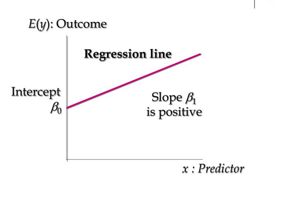
Linear regression models are used to predict the value of one factor based on the value of another factor. The value being predicted is called the dependent variable and the value that is used to predict the dependent variable is called an independent variable. The mathematical equation of linear regression is:
Y=B0+B1 X
Here,
- X: Independent variable
- Y: Dependent variable
- B0: Represents the value of Y when X=0
- B1: Regression Coefficient (this represents the change in the dependent variable based on the unit change in the independent variable)
For example, we can use linear regression to understand whether cigarette consumption can be predicted based on smoking duration. Here, your dependent variable would be “cigarette consumption”, measured in terms of the number of cigarettes consumed daily, and your independent variable would be “smoking duration”, measured in days.
Loss Function
The loss is the error in our predicted value of B0 and B1. Our goal is to minimize this error to obtain the most accurate value of B0 and B1 so that we can get the best fit line for future predictions.
For simplicity, we will use the below loss function:
e(i) = p(i) - y(i)
Here,
- e(i) : error of ith training example
- p(i) : predicted value of ith training example
- y(i): actual value of ith training example
Overview of the Gradient Descent Algorithm
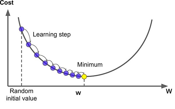
Gradient descent is an iterative optimization algorithm to find the minimum of a function. In our case here, that function is our Loss Function.
Here, our goal is to find the minimum value of the loss function (that is quite close to zero in our case). Gradient descent is an effective algorithm to achieve this. We start with random initial values of our coefficients B0 and B1 and based on the error on each instance, we’ll update their values.
Here’s how it works:
- Initially, let B1 = 0 and B0 = 0. Let L be our learning rate. This controls how much the value of B1 changes with each step. L could be a small value like 0.01 for good accuracy
- We calculate the error for the first point: e(1) = p(1) – y(1)
- We’ll update B0 and B1 according to the following equation:
                                          b0(t+1) = b0(t) - L * error
                                          b1(t+1) = b1(t) - L * error
We’ll do this for each instance of a training set. This completes one epoch. We’ll repeat this for more epochs to get more accurate predictions.
You can refer to these comprehensive guides to get a more in-depth intuition of linear regression and gradient descent:
- A Comprehensive Beginner’s Guide to Linear, Ridge and Lasso Regression
- Introduction to Gradient Descent in Machine Learning
Implementing Linear Regression in C++
Initialization phase:
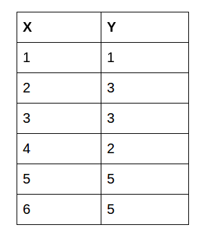
We’ll start by defining our dataset. For the scope of this tutorial, we’ll use this dataset:
We’ll train our dataset on the first 5 values and test on the last value:
Next, we’ll define our variables:
Training Phase
Our next step is the gradient descent algorithm:
Since there are 5 values and we are running the whole algorithm for 4 epochs, hence 20 times our iterative function works. The variable p calculates the predicted value of each instance. The variable err is used for calculating the error of each instance. We then update the values of b0 and b1 as explained above in the gradient descent section above. We finally push the error in the error vector.
As you will notice, B0 does not have any input. This coefficient is often called the bias or the intercept and we can assume it always has an input value of 1.0. This assumption can help when implementing the algorithm using vectors or arrays.
Finally, we’ll sort the error vector to get the minimum value of error and corresponding values of b0 and b1. At last, we’ll print the values:
Testing Phase:
We’ll enter the test value which is 6. The answer we get is 4.9753 which is quite close to 5. Congratulations! We just completed building a linear regression model with C++, and that too with good parameters.
Full Code for final implementation:
Logistic Regression with C++
Logistic Regression is one of the most famous machine learning algorithms for binary classification. This is because it is a simple algorithm that performs very well on a wide range of problems.
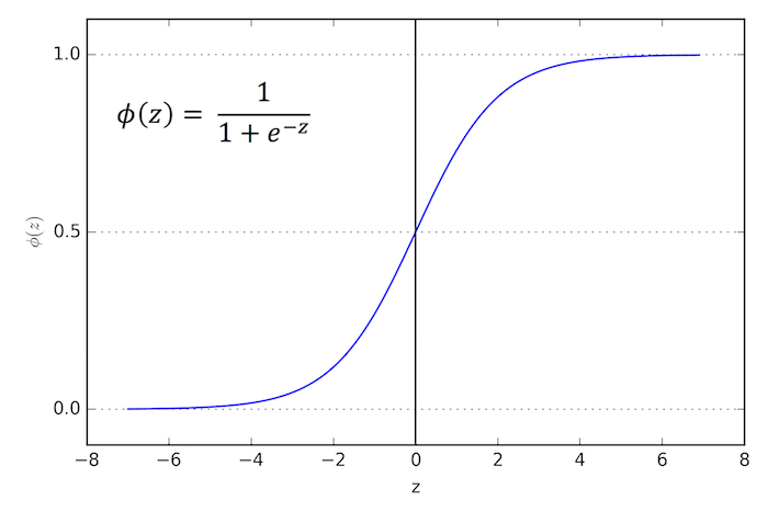
The name of this algorithm is logistic regression because of the logistic function that we use in this algorithm. This logistic function is defined as:
predicted = 1 / (1 + e^-x)
The logistic regression model takes real-valued inputs and makes a prediction as to the probability of the input belonging to the default class (class 0). If the probability is > 0.5 we can take the output as a prediction for the default class (class 0), otherwise, the prediction is for the other class (class 1).
Gradient Descent for Logistic Regression
We can apply stochastic gradient descent to the problem of finding the coefficients for the logistic regression model as follows:
Let us suppose for the example dataset, the logistic regression has three coefficients just like linear regression:
output = b0 + b1*x1 + b2*x2
The job of the learning algorithm will be to discover the best values for the coefficients (b0, b1, and b2) based on the training data.
Given each training instance:
- Calculate a prediction using the current values of the coefficients.
prediction = 1 / (1 + e^(-(b0 + b1*x1 + b2*x2)).
- Calculate new coefficient values based on the error in the prediction. The values are updated according to the below equation:
b = b + alpha * (y – prediction) * prediction * (1 – prediction) * x
Where b is the coefficient we are updating and prediction is the output of making a prediction using the model. Alpha is a parameter that you must specify at the beginning of the training run. This is the learning rate and controls how much the coefficients (and therefore the model) changes or learns each time it is updated.
Like we saw earlier when talking about linear regression, B0 does not have any input. This coefficient is called the bias or the intercept and we can assume it always has an input value of 1.0. So while updating, we’ll multiply with 1.0.
The process is repeated until the model is accurate enough (e.g. error drops to some desirable level) or for a fixed number of iterations.
For a beginner’s guide to logistic regression, check this out – Simple Guide to Logistic Regression.
Implementing Logistic Regression in C++
Initialization phase
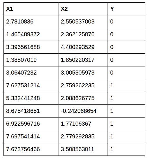
We’ll start by defining the dataset:
We’ll train on the first 10 values and test on the last value:
Next, we’ll initialize the variables:
Training Phase
Since there are 10 values, we’ll run one epoch that takes 10 steps. We’ll calculate the predicted value according to the equation as described above in the gradient descent section:
prediction = 1 / (1 + e^(-(b0 + b1*x1 + b2*x2)))
Next, we’ll update the variables according to the similar equation described above:
b = b + alpha * (y – prediction) * prediction * (1 – prediction) * x
Finally, we’ll sort the error vector to get the minimum value of error and corresponding values of b0, b1, and b2. And finally, we’ll print the values:
Testing phase:
When we enter x1=7.673756466 and x2= 3.508563011, we get pred = 0.59985. So finally we’ll print the class:
So the class printed by the model is 1. Yes! We got the prediction right!
Final Code for full implementation
End Notes
One of the more important steps, in order to learn machine learning, is to implement algorithms from scratch. The simple truth is that if we are not familiar with the basics of the algorithm, we can’t implement that in C++.
This is one of my starting adventures in this field of machine learning with C++. I’m working on more advanced machine learning algorithms so keep an eye out for that!


