Introduction
We have made huge progress in solving Semi Supervised machine learning problems. That also means that we need a lot of data to build our image classifiers or sales forecasters. The algorithms search patterns through the data again and again. In this article, we will introduce you to Pseudo labelling in detail.
But, that is not how human mind learns. A human brain does not require millions of data for training with multiple iterations of going through the same image for understanding a topic. All it needs is a few guiding points to train itself on the underlying patterns. Clearly, we are missing something in current machine learning approaches.
Thankfully, there is a line of research which specifically caters to this question. Can we build a system capable of requiring minimal amount of supervision which can learn majority of the tasks on its own. In this article, I would like to cover one such technique called pseudo-labelling. I will give an intuitive explanation of what pseudo-labelling is and then provide a hands-on implementation of it.
Are you ready?
Note: I assume you have clarity on the basic topics of machine learning. If not, I would suggest you to go through a basic machine learning article first and then come back to this one.
Table of contents
What is Semi-Supervised Learning (SSL) ?
Let’s say, we have a simple image classification problem. So, our training data consists of two labelled images as shown below.
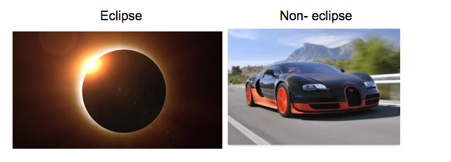
So, we need to classify images of eclipse from the non-eclipse images. But, the problem is that we need to build our model on just a training set of just two images.
Therefore, in order to apply any supervised learning algorithm we need more data to build a robust model. To solve this purpose, we find a simple solution that we download some images from the web to increase our training data.
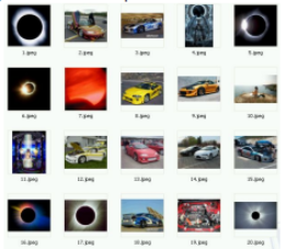
But, for the supervised approach we also need labels for these images. So, we manually classify each image into a category as shown below.
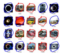
After running supervised algorithm on this data, our model will definitely out-perform the model just containing two images in the training data. But this approach is only valid for small purposes because human annotation to a large dataset can be very hard and expensive.
So, to solve these type of problems, we define a different type of learning known as semi-supervised learning, which is used both labelled data (supervised learning) and unlabelled data (unsupervised learning).
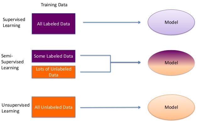
Source: link
Therefore, let us understand how unlabelled data can help to improve our model.
How Unlabelled data can help?
Consider a situation as shown below.
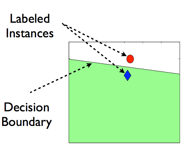
You have only two data points belonging to two different categories, and the line drawn is the decision boundary of any supervised model.
Now, let’s say we add some unlabelled data to this data as shown in the image below.
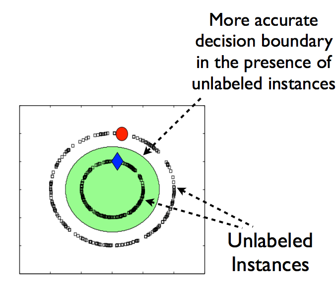
Images source: link
If we notice the difference between the above two images, you can say that after adding unlabelled data, the decision boundary of our model has become more accurate.
So, the advantage of using unlabelled data are:
- Labelled data is expensive and difficult to get while unlabelled is abundant and cheap.
- It improves the model robustness by more precise decision boundary.
Now, we have a basic understanding that what is semi-supervised learning. There are different techniques of applying SSL, in this article we will try to understand one such technique known as Pseudo Labeling.
Introduction Pseudo Labeling
In this technique, instead of manually labeling the unlabelled data, we give approximate labels on the basis of the labelled data. Let’s make it simpler by breaking into steps as shown in the image below.
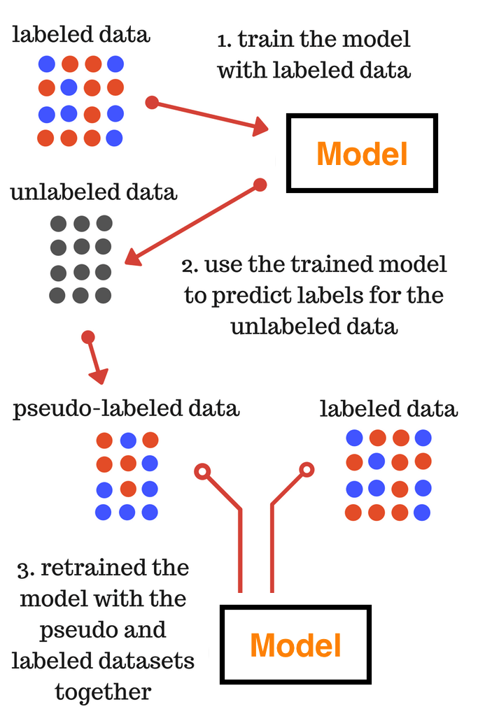
Source: link
I suppose, you understood the steps mentioned in the above image. So, the final model trained in the third step is used for the final predictions on the test data.
For better understanding, I always prefer understanding a concept by its implementation on a real world problem.
Implementation of SSL
Here, we will be using Big Mart Sales problem from AV data hack platform. So, let’s get start by downloading the train and test file present in the data section.
So, let’s get start by importing the basic libraries.
import pandas as pd
import numpy as np
import matplotlib.pyplot as plt
%matplotlib inline
from sklearn.preprocessing import LabelEncoder
Now, let’s read train and test file that we have downloaded and do some basic preprocessing in order to form modelling.

train = pd.read_csv('/Users/shubhamjain/Downloads/AV/Big Mart/train.csv')
test = pd.read_csv('/Users/shubhamjain/Downloads/AV/Big Mart/test.csv')
# preprocessing

### mean imputations
train['Item_Weight'].fillna((train['Item_Weight'].mean()), inplace=True)
test['Item_Weight'].fillna((test['Item_Weight'].mean()), inplace=True)

### reducing fat content to only two categories
train['Item_Fat_Content'] = train['Item_Fat_Content'].replace(['low fat','LF'], ['Low Fat','Low Fat'])
train['Item_Fat_Content'] = train['Item_Fat_Content'].replace(['reg'], ['Regular'])
test['Item_Fat_Content'] = test['Item_Fat_Content'].replace(['low fat','LF'], ['Low Fat','Low Fat'])
test['Item_Fat_Content'] = test['Item_Fat_Content'].replace(['reg'], ['Regular'])

## for calculating establishment year
train['Outlet_Establishment_Year'] = 2013 - train['Outlet_Establishment_Year']
test['Outlet_Establishment_Year'] = 2013 - test['Outlet_Establishment_Year']

### missing values for size
train['Outlet_Size'].fillna('Small',inplace=True)
test['Outlet_Size'].fillna('Small',inplace=True)

### label encoding cate. var.
col = ['Outlet_Size','Outlet_Location_Type','Outlet_Type','Item_Fat_Content']
test['Item_Outlet_Sales'] = 0
combi = train.append(test)
number = LabelEncoder()
for i in col:
 combi[i] = number.fit_transform(combi[i].astype('str'))
 combi[i] = combi[i].astype('int')
train = combi[:train.shape[0]]
test = combi[train.shape[0]:]
test.drop('Item_Outlet_Sales',axis=1,inplace=True)

## removing id variables
training = train.drop(['Outlet_Identifier','Item_Type','Item_Identifier'],axis=1)
testing = test.drop(['Outlet_Identifier','Item_Type','Item_Identifier'],axis=1)
y_train = training['Item_Outlet_Sales']
training.drop('Item_Outlet_Sales',axis=1,inplace=True)

features = training.columns
target = 'Item_Outlet_Sales'

X_train, X_test = training, testing
Starting with different supervised learning algorithm, let us check which algorithm gives us the best results.
from xgboost import XGBRegressor
from sklearn.linear_model import BayesianRidge, Ridge, ElasticNet
from sklearn.neighbors import KNeighborsRegressor
from sklearn.ensemble import RandomForestRegressor, ExtraTreesRegressor, GradientBoostingRegressor
#from sklearn.neural_network import MLPRegressor

from sklearn.metrics import mean_squared_error
from sklearn.model_selection import cross_val_score
model_factory = [
RandomForestRegressor(),
XGBRegressor(nthread=1),
#MLPRegressor(),
Ridge(),
BayesianRidge(),
ExtraTreesRegressor(),
ElasticNet(),
KNeighborsRegressor(),
GradientBoostingRegressor()
]
for model in model_factory:
model.seed = 42
num_folds = 3
scores = cross_val_score(model, X_train, y_train, cv=num_folds, scoring='neg_mean_squared_error')
score_description = " %0.2f (+/- %0.2f)" % (np.sqrt(scores.mean()*-1), scores.std() * 2)
print('{model:25} CV-5 RMSE: {score}'.format(
model=model.__class__.__name__,
score=score_description
))We can see XGB gives us the best model performance. Note here, I have not tuned parameter of any algorithm for the simplicity of this article.
Now, let’s us implement Pseudo-labelling, for this purpose I will be using test data as the unlabelled data.
from sklearn.utils import shuffle
 from sklearn.base import BaseEstimator, RegressorMixin

class PseudoLabeler(BaseEstimator, RegressorMixin):
 '''
 Sci-kit learn wrapper for creating pseudo-lebeled estimators.
 '''

def __init__(self, model, unlabled_data, features, target, sample_rate=0.2, seed=42):
 '''
 @sample_rate - percent of samples used as pseudo-labelled data
 from the unlabelled dataset
 '''
 assert sample_rate <= 1.0, 'Sample_rate should be between 0.0 and 1.0.'

self.sample_rate = sample_rate
 self.seed = seed
 self.model = model
 self.model.seed = seed

self.unlabled_data = unlabled_data
 self.features = features
 self.target = target

def get_params(self, deep=True):
 return {
 "sample_rate": self.sample_rate,
 "seed": self.seed,
 "model": self.model,
 "unlabled_data": self.unlabled_data,
 "features": self.features,
 "target": self.target
 }

def set_params(self, **parameters):
 for parameter, value in parameters.items():
 setattr(self, parameter, value)
 return self

def fit(self, X, y):
 '''
 Fit the data using pseudo labeling.
 '''

augemented_train = self.__create_augmented_train(X, y)
 self.model.fit(
 augemented_train[self.features],
 augemented_train[self.target]
 )

return self


def __create_augmented_train(self, X, y):
 '''
 Create and return the augmented_train set that consists
 of pseudo-labeled and labeled data.
 '''
 num_of_samples = int(len(self.unlabled_data) * self.sample_rate)

# Train the model and creat the pseudo-labels
 self.model.fit(X, y)
 pseudo_labels = self.model.predict(self.unlabled_data[self.features])

# Add the pseudo-labels to the test set
 pseudo_data = self.unlabled_data.copy(deep=True)
 pseudo_data[self.target] = pseudo_labels

# Take a subset of the test set with pseudo-labels and append in onto
 # the training set
 sampled_pseudo_data = pseudo_data.sample(n=num_of_samples)
 temp_train = pd.concat([X, y], axis=1)
 augemented_train = pd.concat([sampled_pseudo_data, temp_train])

return shuffle(augemented_train)

def predict(self, X):
 '''
 Returns the predicted values.
 '''
 return self.model.predict(X)

def get_model_name(self):
 return self.model.__class__.__name__
This look quite complex, but you need not to worry about this as it is the same implementation of the method. So, copy the same code every time you need to perform pseudo labeling.
So, now let’s us now check the results of pseudo labeling on the dataset.
model_factory = [
 XGBRegressor(nthread=1),
 PseudoLabeler(
 XGBRegressor(nthread=1),
 test,
 features,
 target,
 sample_rate=0.3
 ),
]

for model in model_factory:
 model.seed = 42
 num_folds = 8

 scores = cross_val_score(model, X_train, y_train, cv=num_folds, scoring='neg_mean_squared_error', n_jobs=8)
 score_description = "MSE: %0.4f (+/- %0.4f)" % (np.sqrt(scores.mean()*-1), scores.std() * 2)

print('{model:25} CV-{num_folds} {score_cv}'.format(
 model=model.__class__.__name__,
 num_folds=num_folds,
 score_cv=score_description
 ))
In this case, we a get rmse value which comes out to lesser than any of the supervised learning algorithm.
If you have notice sample_rate was one of the parameter, which denotes the percentage of unlabelled data to be used as the pseudo labelled for the modelling purpose.
Therefore, let’s us check the dependance of sample_rate on the performance of the pseudo labelling.
Dependence of Sampling Rate
In order to find out the dependence of sample_rate on the performance of the pseudo labelling, let us plot a graph between those two.
Here, I am using only two algorithm to show you the dependence because of the time constraint, but you can try for other algorithms too.
sample_rates = np.linspace(0, 1, 10)

def pseudo_label_wrapper(model):
 return PseudoLabeler(model, test, features, target)

# List of all models to test
model_factory = [
 RandomForestRegressor(n_jobs=1),
 XGBRegressor(),
]

# Apply the PseudoLabeler class to each model
model_factory = map(pseudo_label_wrapper, model_factory)

# Train each model with different sample rates
results = {}
num_folds = 5

for model in model_factory:
 model_name = model.get_model_name()
 print('%s' % model_name)

results[model_name] = list()
 for sample_rate in sample_rates:
 model.sample_rate = sample_rate

 # Calculate the CV-3 R2 score and store it
 scores = cross_val_score(model, X_train, y_train, cv=num_folds, scoring='neg_mean_squared_error', n_jobs=8)
 results[model_name].append(np.sqrt(scores.mean()*-1))
plt.figure(figsize=(16, 18))

i = 1
for model_name, performance in results.items():
 plt.subplot(3, 3, i)
 i += 1

 plt.plot(sample_rates, performance)
 plt.title(model_name)
 plt.xlabel('sample_rate')
 plt.ylabel('RMSE')


plt.show()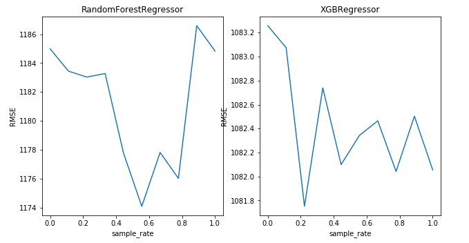
So, we can see that the rmse is minimum for a particular value of sample_rate, which is different for both the algorithm.
Therefore, it is important to tune sample_rate in order to achieve better results while using pseudo labeling.
Applications of SSL
In past, there are limited number of applications of semi-supervised learning, but currently there is lot of working going on in this field.
Some interesting applications are:
1. Multimodal semi-supervised learning for image classification
Generally, in image categorisation, the goal is to classify an image whether it belongs to the category or not. In this paper, not only images are used for modelling but the keywords associated with labelled and unlabelled images to improve the classifier using semi-supervised learning.

Source: link
2. SSL for detecting human trafficking
Human trafficking is one of the most atrocious crimes and among the challenging problems facing law enforcement which demands attention of global magnitude. Semi-supervised learning is to applied to use both labelled and unlabelled data in order to produce better results than the normal approaches.
End Notes
I hope that now you have a understanding what semi-supervised learning is and how to implement it in any real world problem. Therefore, try to explore it further and learn other types of semi-supervised learning technique/ machine learning techniques and share with the community in the comment section.
You can find the full code of this article from my github repository.
Also, did you find this article helpful? Please share your opinions / thoughts in the comments section below.


