An Introduction to the Powerful Bayes’ Theorem for Data Science Professionals

Overview

• Bayes’ Theorem is one of the most powerful concepts in statistics – a must-know for data science professionals
• Get acquainted with Bayes’ Theorem, how it works, and its multiple and diverse applications
• Plenty of intuitive examples in this article to grasp the idea behind Bayes’ Theorem

Introduction

Probability is at the very core of a lot of data science algorithms. In fact, the solutions to so many data science problems are probabilistic in nature – hence I always advice focusing on learning statistics and probability before jumping into the algorithms.

But I’ve seen a lot of aspiring data scientists shunning statistics, especially Bayesian statistics. It remains incomprehensible to a lot of analysts and data scientists. I’m sure a lot of you are nodding your head at this!

Bayes’ Theorem, a major aspect of Bayesian Statistics, was created by Thomas Bayes, a monk who lived during the eighteenth century. The very fact that we’re still learning about it shows how influential his work has been across centuries! Bayes’ Theorem enables us to work on complex data science problems and is still taught at leading universities worldwide.

In this article, we will explore Bayes’ Theorem in detail along with its applications, including in Naive Bayes’ Classifiers and Discriminant Functions, among others. There’s a lot to unpack in this article so let’s get going!

Table of Contents

• Prerequisites for Bayes’ Theorem
• What is Bayes’ Theorem?
• An Illustration of Bayes’ Theorem
• Applications of Bayes’ Theorem
  • Naive Bayes’ Classifiers
  • Discriminant Functions and Decision Surfaces
  • Bayesian Parameter Estimation
• Demonstration of Bayesian Parameter Estimation

Prerequisites for Bayes’ Theorem

We need to understand a few concepts before diving into the world of Bayes’ Theorem. These concepts are essentially the prerequisites for understanding Bayes’ Theorem.

1. Experiment

What’s the first image that comes to your mind when you hear the word “experiment”? Most people, including me, imagine a chemical laboratory filled with test tubes and beakers. The concept of an experiment in probability theory is actually quite similar:

An experiment is a planned operation carried out under controlled conditions.

Tossing a coin, rolling a die, and drawing a card out of a well-shuffled pack of cards are all examples of experiments.

2. Sample Space

The result of an experiment is called an outcome. The set of all possible outcomes of an event is called the sample space. For example, if our experiment is throwing dice and recording its outcome, the sample space will be:

S1 = {1, 2, 3, 4, 5, 6}

What will be the sample when we’re tossing a coin? Think about it before you see the answer below:

S2 = {H, T}

3. Event

An event is a set of outcomes (i.e. a subset of the sample space) of an experiment.

Let’s get back to the experiment of rolling a dice and define events E and F as:

• E = An even number is obtained = {2, 4, 6}
• F = A number greater than 3 is obtained = {4, 5, 6}

The probability of these events:

P(E) = Number of favourable outcomes / Total number of possible outcomes = 3 / 6 = 0.5
P(F) = 3 / 6 = 0.5

The basic operations in set theory, union and intersection of events, are possible because an event is a set.

Then, E∪F = {2, 4, 5, 6} and E∩F = {4, 6}

Now consider an event G = An odd number is obtained:

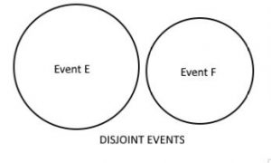
Then E ∩ G = empty set = Φ

Such events are called disjoint events. These are also called mutually exclusive events because only one out of the two events can occur at a time:

4. Random Variable

A Random Variable is exactly what it sounds like – a variable taking on random values with each value having some probability (which can be zero). It is a real-valued function defined on the sample space of an experiment:

Source: Wikipedia

Let’s take a simple example (refer to the above image as we go along). Define a random variable X on the sample space of the experiment of tossing a coin. It takes a value +1 if “Heads” is obtained and -1 if “Tails” is obtained. Then, X takes on values +1 and -1 with equal probability of 1/2.

Consider that Y is the observed temperature (in Celsius) of a given place on a given day. So, we can say that Y is a continuous random variable defined on the same space, S = [0, 100] (Celsius Scale is defined from zero degree Celsius to 100 degrees Celsius).

5. Exhaustive Events

A set of events is said to be exhaustive if at least one of the events must occur at any time. Thus, two events A and B are said to be exhaustive if A ∪ B = S, the sample space.

For example, let’s say that A is the event that a card drawn out of a pack is red and B is the event that the card drawn is black. Here, A and B are exhaustive because the sample space S = {red, black}. Pretty straightforward stuff, right?

6. Independent Events

If the occurrence of one event does not have any effect on the occurrence of another, then the two events are said to be independent. Mathematically, two events A and B are said to be independent if:

P(A ∩ B) = P(AB) = P(A)*P(B)

For example, if A is obtaining a 5 on throwing a die and B is drawing a king of hearts from a well-shuffled pack of cards, then A and B are independent just by their definition. It’s usually not as easy to identify independent events, hence we use the formula I mentioned above.

7. Conditional Probability

Consider that we’re drawing a card from a given deck. What is the probability that it is a black card? That’s easy – 1/2, right? However, what if we know it was a black card – then what would be the probability that it was a king?

The approach to this question is not as simple.

This is where the concept of conditional probability comes into play. Conditional probability is defined as the probability of an event A, given that another event B has already occurred (i.e. A conditional B). This is represented by P(A|B) and we can define it as:

P(A|B) = P(A ∩ B) / P(B)

Let event A represent picking a king, and event B, picking a black card. Then, we find P(A|B) using the above formula:

P(A ∩ B) = P(Obtaining a black card which is a King) = 2/52 
P(B) = P(Picking a black card) = 1/2

Thus, P(A|B) = 4/52. Try this out on an example of your choice. This will help you grasp the entire idea really well.

8. Marginal Probability

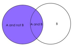
It is the probability of an event A occurring, independent of any other event B, i.e. marginalizing the event B.

Marginal probability P(A) = P(A|B)*P(B) + P(A|~B)*P(~B)

This is just a fancy way of saying:

P(A) = P(A ∩ B) + P(A ∩ ~B)   #from our knowledge of conditional probability

where ~B represents the event that B does not occur.

Let’s check if this concept of marginal probability holds true. Here, we need to calculate the probability that a random card drawn out of a pack is red (event A). The answer is obviously 1/2. Let’s calculate the same through marginal probability with event B as drawing a king.

P(A ∩ B) = 2/52 (because there are 2 kings in red suits, one of hearts and other of diamonds)

Source: Itembrowser.com

and P(A ∩ ~B) = 24/52 (remaining cards from the red suit)
Therefore, P(A) = 2/52 + 24/52 = 26/52 = 1/2

Perfect! So this is good enough to cover our basics of Bayes’ Theorem. Let’s now take a few moments to understand what exactly Bayes’ Theorem is and how it works.

What is Bayes’ Theorem?

Have you ever seen the popular TV show ‘Sherlock’ (or any crime thriller show)? Think about it – our beliefs about the culprit change throughout the episode. We process new evidence and refine our hypothesis at each step. This is Bayes’ Theorem in real life!

Now, let’s understand this mathematically. This will be pretty simple now that our basics are clear.

Consider that A and B are any two events from a sample space S where P(B) ≠ 0. Using our understanding of conditional probability, we have:

 P(A|B) = P(A ∩ B) / P(B)
Similarly, P(B|A) = P(A ∩ B) / P(A)
It follows that P(A ∩ B) = P(A|B) * P(B) = P(B|A) * P(A)
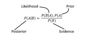
Thus, P(A|B) = P(B|A)*P(A) / P(B)

This is the Bayes’ Theorem.

Here, P(A) and P(B) are probabilities of observing A and B independently of each other. That’s why we can say that they are marginal probabilities. P(B|A) and P(A|B) are conditional probabilities.

P(A) is called Prior probability and P(B) is called Evidence.

P(B) = P(B|A)*P(A) + P(B|~A)*P(~A)

P(B|A) is called Likelihood and P(A|B) is called Posterior probability.

Equivalently, Bayes Theorem can be written as:

posterior = likelihood * prior / evidence

These words might sound fancy but the underlying idea behind them is really simple. You can always refer back to this section whenever you have any doubts or reach out to me directly in the comments section below.

An Illustration of Bayes’ Theorem

Let’s solve a problem using Bayes’ Theorem. This will help you understand and visualize where you can apply it. We’ll take an example which I’m sure almost all of us have seen in school.

There are 3 boxes labeled A, B, and C:

• Box A contains 2 red and 3 black balls
• Box B contains 3 red and 1 black ball
• And box C contains 1 red ball and 4 black balls

The three boxes are identical and have an equal probability of getting picked. Consider that a red ball is chosen. Then what is the probability that this red ball was picked out of box A?

Source: i.ytimg.com

Let E denote the event that a red ball is chosen and A, B, and C denote that the respective box is picked. We are required to calculate the conditional probability P(A|E).

We have prior probabilities P(A) = P(B) = P (C) = 1 / 3, since all boxes have equal
probability of getting picked.

P(E|A) = Number of red balls in box A / Total number of balls in box A = 2 / 5
Similarly, P(E|B) = 3 / 4 and P(E|C) = 1 / 5

Then evidence P(E) = P(E|A)*P(A) + P(E|B)*P(B) + P(E|C)*P(C) 
                   = (2/5) * (1/3) + (3/4) * (1/3) + (1/5) * (1/3) = 0.45
Therefore, P(A|E) = P(E|A) * P(A) / P(E) = (2/5) * (1/3) / 0.45 = 0.296

Applications of Bayes’ Theorem

There are plenty of applications of the Bayes’ Theorem in the real world. Don’t worry if you do not understand all the mathematics involved right away. Just getting a sense of how it works is good enough to start off.

Bayesian Decision Theory is a statistical approach to the problem of pattern classification. Under this theory, it is assumed that the underlying probability distribution for the categories is known. Thus, we obtain an ideal Bayes Classifier against which all other classifiers are judged for performance.

We will discuss the three main applications of Bayes’ Theorem:

• Naive Bayes’ Classifiers
• Discriminant Functions and Decision Surfaces
• Bayesian Parameter Estimation

Let’s look at each application in detail.

Naive Bayes’ Classifiers

This is probably the most famous application of Bayes’ Theorem, probably even the most powerful. You’ll come across the Naive Bayes algorithm a lot in machine learning.

Naive Bayes’ Classifiers are a set of probabilistic classifiers based on the Bayes’ Theorem. The underlying assumption of these classifiers is that all the features used for classification are independent of each other. That’s where the name ‘naive’ comes in since it is rare that we obtain a set of totally independent features.

The way these classifiers work is exactly how we solved in the illustration, just with a lot more features assumed to be independent of each other.

Here, we need to find the probability P(Y|X) where X is an n-dimensional random variable whose component random variables X_1, X_2, …., X_n are independent of each other:

Finally, the Y for which P(Y|X) is maximum is our predicted class.

Let’s talk about the famous Titanic dataset. We have the following features:

Remember the problem statement? We need to calculate the probability of survival conditional to all the other variables available in the dataset. Then, based on this probability, we predict if the person survived or not, i.e, class 1 or 0.

This is where I pass the buck to you. Refer to our popular article to learn about these Naive Bayes classifiers along with the relevant code in both Python and R, and try solving the Titanic dataset yourself.

You can also enrol in our free course to learn about this interesting algorithm in a structured way: Naive Bayes from Scratch

If you get stuck anywhere, you can find me in the comments section below!

Discriminant Functions and Surfaces

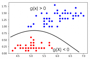
The name is pretty self-explanatory. A discriminant function is used to “discriminate” its argument into its relevant class. Want an example? Let’s take one!

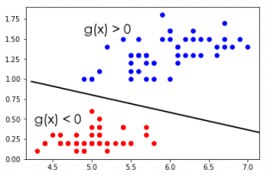
You might have come across Support Vector Machines (SVM) if you have explored classification problems in machine learning. The SVM algorithm classifies the vectors by finding the differentiating hyperplane which best segregates our training examples. This hyperplane can be linear or non-linear:

These hyperplanes are our decision surfaces and the equation of this hyperplane is our discriminant function. Make sure you check out our article on Support Vector Machine. It is thorough and includes code both in R and Python.

Alright – now let’s discuss the topic formally.

Let w_1, w_2, ….., w_c denote the c classes that our data vector X can be classified into. Then the decision rule becomes:

Decide w_i if g_i(X) > g_j(X) for all j ≠ i

These functions g_i(X), i = 1, 2, …., c, are known as Discriminant functions. These functions separate the vector space into c decision regions – R_1, R_2, …., R_c corresponding to each of the c classes. The boundaries of these regions are called decision surfaces or boundaries.

If g_i(X) = g_j(X) is the largest value out of the c discriminant functions, then the classification of vector X into class w_i and w_j is ambiguous. So, X is said to lie on a decision boundary or surface.

Check out the below figure:

Source: Duda, R. O., Hart, P. E., & Stork, D. G. (2012). Pattern classification. John Wiley & Sons.

It’s a pretty cool concept, right? The 2-dimensional vector space is separated into two decision regions, R_1 and R_2, separated by two hyperbolas.

Note that any function f(g_i(X)) can also be used as a discriminant function if f(.) is a monotonically increasing function. The logarithm function is a popular choice for f(.).

Now, consider a two-category case with classes w _1 and w_2. The ‘minimum error-rate classification‘ decision rule becomes:

Decide w_1 if P(w_1|X) > P(w_2|X), otherwise decide w_2
with P(error|X) = min{P(w_1|X), P(w_2|X)}

P(w_i|X) is a conditional probability and can be calculated using Bayes’ Theorem. So, we can restate the decision rule in terms of likelihoods and priors to get:

 Decide w_1 if P(X|w_1)*P(w_1) > P(X|w_2)*P(w_2), otherwise decide w_2

Notice that the ‘evidence’ on the denominator is merely used for scaling and hence we can eliminate it from the decision rule.

Thus, an obvious choice for the discriminant functions is:

g_i(X) = P(X|w_i)*P(w_i) OR
g_i(X) = ln(P(X|w_i)) + ln(P(w_i))

The 2-category case can generally be classified using a single discriminant function.

g(X) = g_1(X) - g_2(X)
     = ln(P(X|w_1) / P(X|w_2)) + ln(P(w_1) / P(w_2))

Decide w_1, if g(X) > 0
Decide w_2, if g(X) < 0
if g(X) = 0, X lies on the decision surface.

In the figure above, g(X) is a linear function in a 2-dimensional vector X. However, more complicated decision boundaries are also possible:

Bayesian Parameter Estimation

This is the third application of Bayes’ Theorem. We’ll use univariate Gaussian Distribution and a bit of mathematics to understand this. Don’t worry if it looks complicated – I’ve broken it down into easy-to-understand terms.

You must have heard about the ultra-popular IMDb Top 250. This is a list of 250 top-rated movies of all time. Shawshank Redemption is #1 on the list with a rating of 9.2/10.

How do you think these ratings are calculated? The original formula used by IMDb claimed to use a “true Bayesian estimate”. The formula has since changed and is not publicly disclosed. Nonetheless, here is the previous formula:

Source: Wikipedia

The final rating W is a weighted average of R and C with weights v and m respectively. m is a prior estimate.

• As the number of votes, v, increases and surpasses m, the minimum votes required, W, approaches the straight average for the movie, R
• As v gets closer to zero (less number of votes are cast for the movie), W approaches the mean rating for all films, C

We generally do not have complete information about the probabilistic nature of a classification problem. Instead, we have a vague idea of the situation along with a number of training examples. We then use this information to design a classifier.

The basic idea is that the underlying probability distribution has a known form. We can, therefore, describe it using a parameter vector Θ. For example, a Gaussian distribution can be described by Θ  = [μ, σ²].

Source: Wikipedia

Then, we need to estimate this vector. This is generally achieved in two ways:

• Maximum Likelihood Estimation (MLE): The assumption is that the underlying probability distribution p(Θ) has an unknown but fixed parameter vector. The best estimate maximizes the likelihood function:

p(D|θ) = p(x1|θ) * p(x2|θ) * ....* p(xn|θ) = Likelihood of θ with respect to the set of samples D

I recommend reading this article to get an intuitive and in-depth explanation of maximum likelihood estimation along with a case study in R.

• Bayesian Parameter Estimation – In Bayesian Learning, Θ is assumed to be a random variable as opposed to an “unknown but fixed” value in MLE. We use training examples to convert a distribution on this variable into a posterior probability density.

We can write it informally as:

P(Θ|data) = P(data|Θ)*P(Θ) / P(data), where data represents the set of training examples

Key points you should be aware of:

1. We assume that the probability density p(X) (samples are drawn from this probability rule) is unknown but has a known parametric form. Thus, it can be said that p(X|Θ) is completely known
2. Any prior information that we might have about Θ is contained in a known prior probability density p(Θ)
3. We use training samples to find the posterior density p(Θ|data). This should sharply peak at the true value of Θ

Demonstration of Bayesian Parameter Estimation – Univariate Gaussian Case

Let me demonstrate how Bayesian Parameter Estimation works. This will provide further clarity on the theory we just covered.

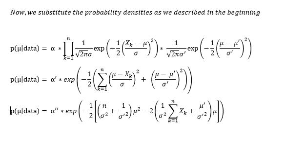
First, let p(X) be normally distributed with a mean μ and variance σ², where μ is the only unknown parameter we wish to estimate. Then:

p(X|Θ) = p(X|μ) ~ N(μ, σ²)

We’ll ease up on the math here. So, let prior probability density p(μ) also be normally distributed with mean µ’ and variance σ’² (which are both known).

Here, p(Θ|data) = p(μ|data) is called the reproducing density and p(Θ) =  p(μ) is called the conjugate prior.

Since this argument in exp() is quadratic in μ, it represents a normal density. Thus, if we have n training examples, we can say that p(μ|data) is normally distributed with mean μ_n and variance σ_n², where

My observations:

1. As n increases, σ_n² decreases. Hence, uncertainty in our estimate decreases
2. Since uncertainty decreases, the density curve becomes sharply peaked at its mean μ_n:

Source: spcforexcel.com

Here’s a superb and practical implementation of Bayesian Statistics and estimation:

• Bayesian Statistics explained to Beginners in Simple English

End Notes

The beauty and power of Bayes’ Theorem never cease to amaze me. A simple concept, given by a monk who died more than 250 years ago, has its use in some of the most prominent machine learning techniques today.

You might have a few questions on the various mathematical aspects we explored here. Feel free to connect with me in the comments section below and let me know your feedback on the article as well.