This article was published as a part of the Data Science Blogathon
Overview
In this article, we will learn the working of the Support Vector Machine algorithm (SVM) and the implementation of SVM by taking an example dataset, building a Classification model in Python.
Intro
A simple question to think of, when do we use Classification? In Machine learning, Classification refers to the process of classifying/predicting a multiclass categorical variable for the given input data. Some examples of classification problems are spam detection, sentiment analysis, animal breed classification, etc.
The popular Classification algorithms are:
- Logistic Regression
- Naive Bayes
- K-Nearest Neighbours
- Decision Trees
- Random Forest
- Support Vector Machine
We will be focussing on the Support Vector Machine (SVM) algorithm in this article.
Support Vector Machine (SVM) algorithm
Support Vector Machine aka Support Vector Network is a supervised machine learning algorithm used for classification and regression problems.
Terminology
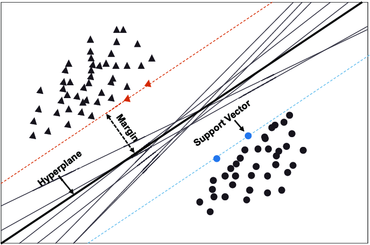
Hyperplane: A hyperplane aka decision boundary/surface is an n-dimensional Euclidean space that distinctly separates the data points. The data points on either side of the hyperplane belong to different classes. If we have a p-dimensional feature set, the dimension of the hyperplane will be p-1.
Support Vectors: The individual data points that are close to the hyperplane are called the support vectors.
Margin: The width that the boundary could be increased before hitting a data point. In simple terms, the distance between the hyperplane and the support vectors is referred to as the Margin.
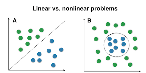
Linear separability: A dataset is linearly separable if there is at least one line that clearly distinguishes the classes.
Non-linear separability: A dataset is said to be non-linearly separable if there isn’t a single line that clearly distinguishes the classes.
How does SVM work?
In SVM, the data of finite-dimensional space is mapped to much a higher dimension (p-dimension) and aims at finding the p-1 dimension hyperplane called a linear classifier.
If the data is linearly separable, unlike logistic regression, in addition to finding the p-1 dimension hyperplane, SVM creates two parrel hyperplanes on either side that passes through the nearest data points(Support Vectors). The region bounded by these two hyperplanes is called the margin.
There could be many such hyperplanes that can be drawn to classify the data. The stablest hyperplane is the one that has the maximum margin. Margin is the distance between the two classes. The hyperplane that has the maximum margin is called the maximum margin hyperplane and the classifier it defines is known as the maximum margin classifier. Now take a look at the image below for a better understanding.
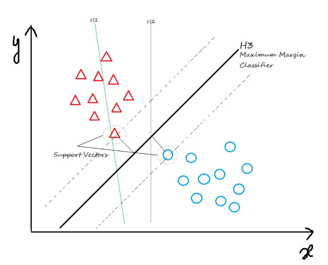
In the above figure, the hyperplane H1 doesn’t classify the datapoints, H2 classifies the data points but has the least marginal width. The hyperplane H3 is the best or optimal classifier as it well classifies the data points and has the highest marginal width.
To sum it up in simple terms, SVM is basically used to linearly separate the classes of the output variable by drawing a Classifier/hyperplane — for a 2D space, the hyperplane is a Line; for a 3D space, a hyperplane is a Plane.
Imagine we have non-linear separable data. How do we classify them?
In this case, we cannot have a linear hyperplane to separate the two classes. So, how does SVM solve this kind of problem?
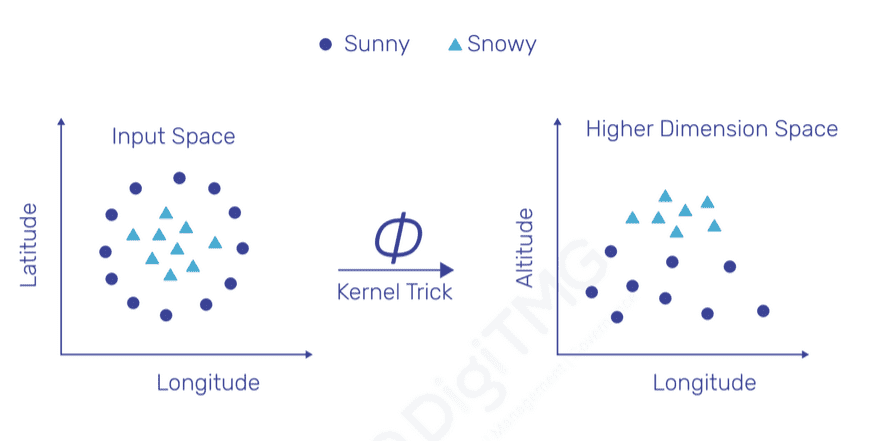
If the data is non-linearly separable, we need to apply transformations that map the original data to a much higher dimensional space. After transformation, the data would be linearly separable and we can easily find a hyperplane/decision boundary to classify.
If we have a manageable number of features, we can manually try some transformation techniques to convert non-linear data to become linearly separable. But what if we have thousands of features? The computational time would go up, and it is humanly impossible to manually handle all those features. Thus, it can be achieved by a key feature called the Kernel trick.
After the trick has been applied, the Latitude is mapped to a new dimension called Altitude. So, it is Latitude versus Longitude mapped to Altitude versus Longitude.
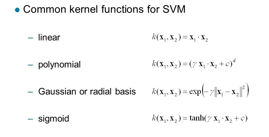
Popular SVM Kernel functions:
1. Linear Kernel: It is just the dot product of all the features. It doesn’t transform the data.
2. Polynomial Kernel: It is a simple non-linear transformation of data with a polynomial degree added.
3. Gaussian Kernel: It is the most used SVM Kernel for usually used for non-linear data.
4. Sigmoid Kernel: It is similar to the Neural Network with sigmoid activation function.
In simple terms, a kernel is nothing but a transformation that we apply to the existing features so that we can draw a classifier easily for non-linearly separable datapoints.
Till now, we have understood the working of the SVM algorithm. Let’s take an example dataset and see the implementation in Python.
SVM implementation in Python
Here, we are going to use the Fish dataset from Kaggle. I have downloaded the dataset and added it to my Github repository for easy access.
Here is how to add a file to the Github repository and Read CSV data from Github.
The Fish data set has 7 features: Species, Weight, Length1, Length2, Length3, Height, and Width.
We aim to predict the ‘Species’ based on the rest of the features. Species is a multi-class categorical variable holding the labels ‘Bream’, ‘Roach’, ‘Whitefish’, ‘Parkki’, ‘Perch’, ‘Pike’, ‘Smelt’.
Steps by step implementation:
Install necessary modules
!pip install pandas sklearn
Import necessary modules
import pandas as pd
from sklearn.model_selection import train_test_split
from sklearn.svm import SVC
Create a pandas dataframe from the Fish dataset
dataset_url = "https://raw.githubusercontent.com/harika-bonthu/SupportVectorClassifier/main/datasets_229906_491820_Fish.csv"
fish = pd.read_csv(dataset_url)
fish
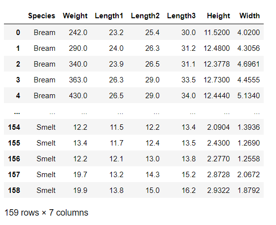
Our dataset has a total of 159 observations and 7 features.
Define the Feature and the Target variables
X = fish.drop(['Species'], axis = 'columns')
y = fish.Species
Split the data into train, test sets using train_test_split
X_train, X_test, y_train, y_test = train_test_split(X, y, test_size= 0.2)
Instantiate Linear SVC object
model = SVC(kernel = 'linear', C = 1)
Train the linear SVC classifier using the training data
model.fit(X_train, y_train)
Make predictions
svm_pred = model.predict(X_test)
Check the accuracy of the model using the scoring method
accuracy = model.score(X_test, y_test)
accuracy

Note: Classifier accuracy is calculated as score(X, y, sample_weight=None). Unlike other accuracy methods, the “score” method takes raw input X_test and predicts the output, and then calculates the accuracy by comparing the output with y_test. The classifier score method calls predict on their own so don’t get confused while calculating the accuracy.
Finally, we built a model that scored 96% accuracy. Just try playing around with the hyperparameters like C(regularization), gamma to see if we can get better accuracy.
Complete Python code for implementing SVM
!pip install pandas sklearn
import pandas as pd
from sklearn.model_selection import train_test_split
from sklearn.svm import SVC

dataset_url = "https://raw.githubusercontent.com/harika-bonthu/SupportVectorClassifier/main/datasets_229906_491820_Fish.csv"
fish = pd.read_csv(dataset_url)
X = fish.drop(['Species'], axis = 'columns')
y = fish.Species

X_train, X_test, y_train, y_test = train_test_split(X, y, test_size= 0.2)

model = SVC(kernel = 'linear', C = 1)

model.fit(X_train, y_train)
svm_pred = model.predict(X_test)
accuracy = model.score(X_test, y_test)
End Notes
By the end of this article, I hope we have got a basic understanding of the working of the SVM algorithm. We have also seen the step-by-step implementation of the SVM algorithm in Python by taking an example Kaggle dataset.
References
Read more about SVM from here
Support Vector Classification Documentation
Check out the Jupyter Notebook from my GitHub repo


