4 ways to compare two columns in Microsoft Excel

Microsoft Excel worksheets can become complicated, especially when comparing columns for validation. Manually cross-checking large datasets on your personal computer may cause you to overlook details and produce errors. You could use Excel’s Visual Basic editor and VBA code to create macros that automate tasks and perform complex calculations. But that requires technical knowledge that not everyone has. There are simpler ways, and we show you the best ones.

How to compare Microsoft Excel columns with the IF function

The IF Excel formula is a logical function that checks conditions and returns a value based on the outcome. In this case, the conditions are the rows in the columns you want to compare. If a row matches, the condition is true. If the function can’t find matches, the conditions are false.

Let’s use a spreadsheet with two columns as an example. Column A contains products that have run out of stock, and Column B shows the stocked items in inventory. To compare both columns and see if a product is in stock, we’ll insert the IF function in Column C or other cells and establish a match between the unavailable and stocked products. Here’s how to do it:

1. From your computer browser, visit office.com/launch/Excel and open a spreadsheet.
2. Click the cell where you’ll type the formula and display the result.
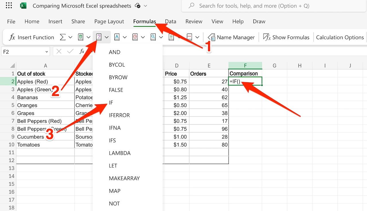
3. Go to the Formulas tab and select Logical (the book icon with a red question mark). Then, select IF from the drop-down list of functions. The function appears in your selected cell.

4. 

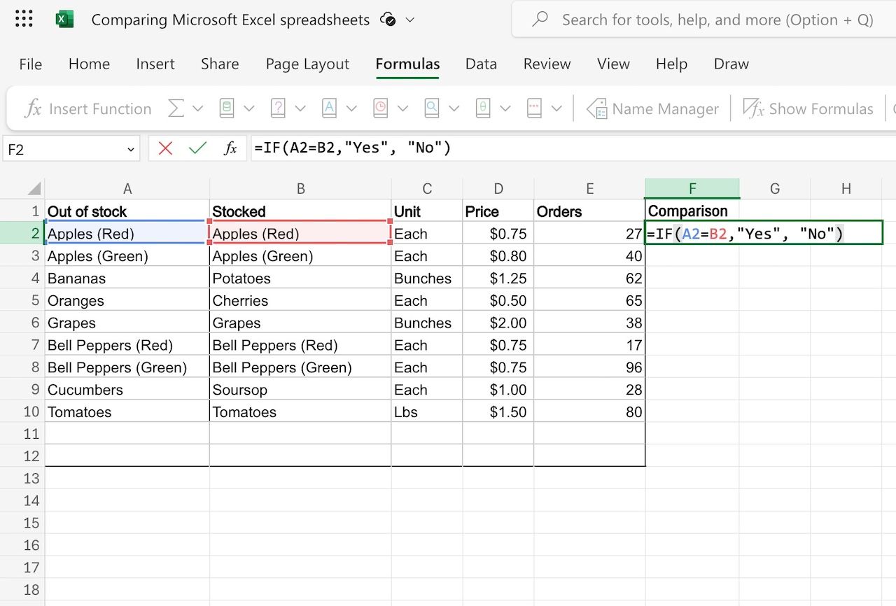
   Double-click the cell to edit the formula.

5. Place your mouse cursor in the bracket.
6. Type the cells you want to compare, separated by the equal sign. For example, A2=B2.
7. Type a comma (,) followed by the value you want the function to produce in quotes. For example, “Yes” or “Match” and “No” or “Mismatch”.

   

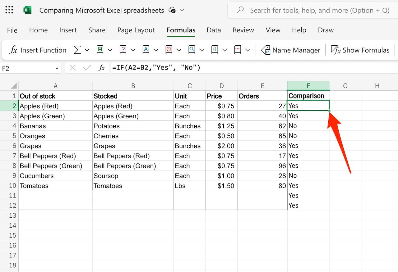
8. Press Enter on your keyboard to complete the function.
9. Drag the lower-right edge of the cell containing the result across the cells underneath it. This action applies the appropriate values to them.

   

Related

How to enable or disable Excel macros

Be aware of security risks when dealing with Excel macros

How to compare Microsoft Excel columns with the EXACT function

EXACT is a text-based function in Microsoft Excel. It’s a stickler for details compared to the IF function. Use it to confirm that columns match perfectly, down to the big and small characters. For example, the function produces a FALSE value when a spreadsheet contains the word Android and the capitalized ANDROID variation.

If you store passwords in spreadsheets, it’s an effective method to cross-check them for case-sensitive mismatches. Here’s how to apply the EXACT function in column comparisons:

1. From your computer browser, visit office.com/launch/Excel and open a spreadsheet.
2. Click the cell where you’ll type the formula and display the result.
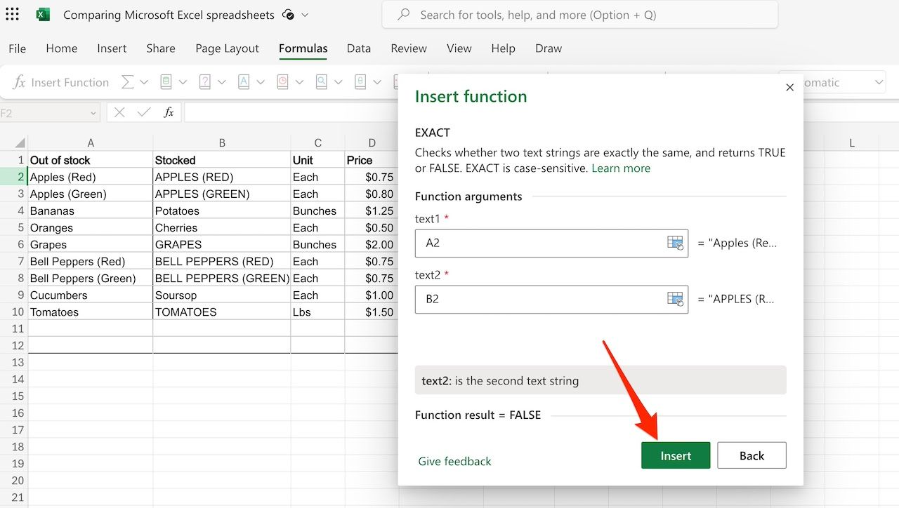
3. Go to Formulas > Text and select EXACT from the functions list. A new window pops up.
4. Click the cells you want to compare to enter their text into the provided boxes automatically.
5. Click Insert.

   

6. Drag the lower-right edge of the cell containing the result across the cells underneath it. This action applies the appropriate values to them.

How to compare Microsoft Excel columns with conditional formatting

Use conditional formatting to highlight column and row differences with colors or other formatting options. This way, you can spot them easily. Follow the steps below to use it:

1. With an Excel spreadsheet open, click the search bar at the top of the screen and enter Conditional formatting.
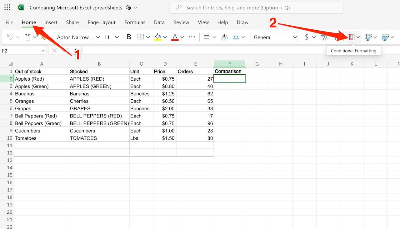
2. Alternatively, click the Home tab from the options above the spreadsheet. Then, click the conditional formatting icon on the right side of the toolbar.

   

3. Click Highlight cell rules.
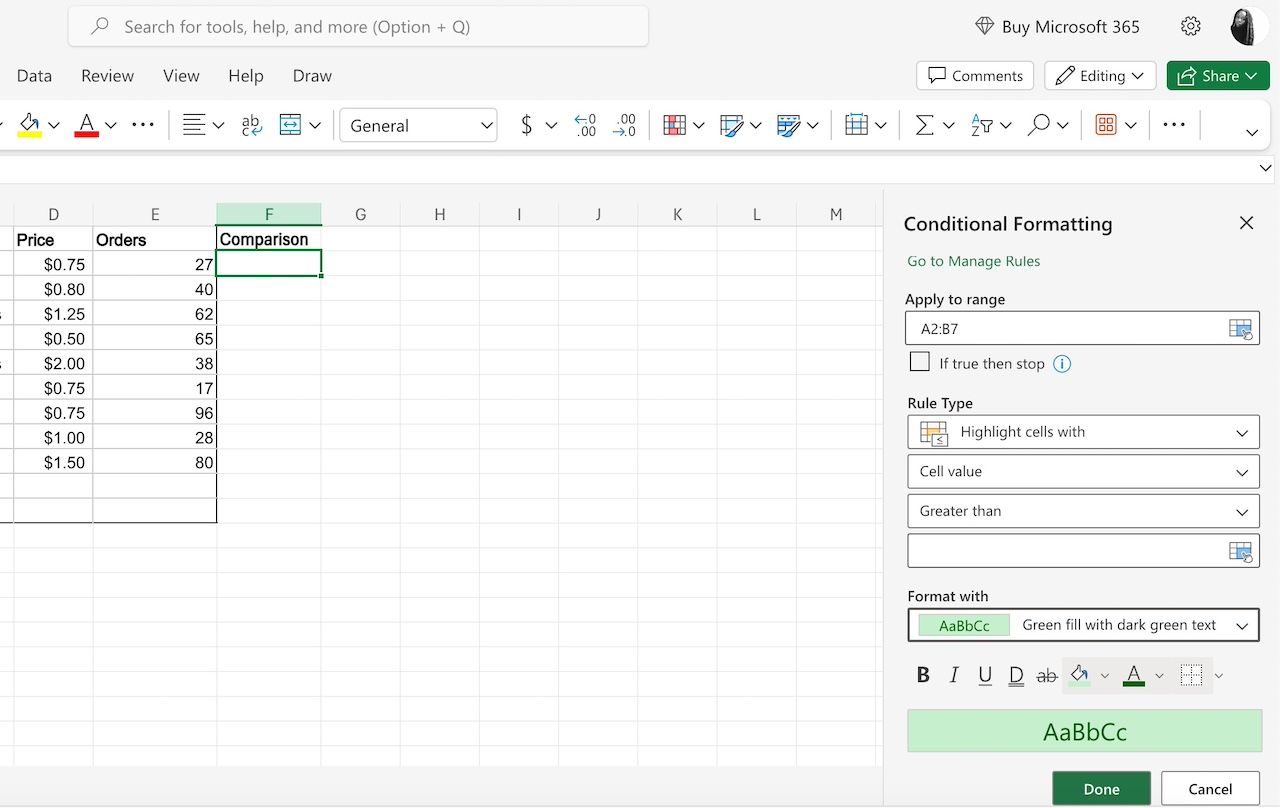
4. Use the expanded options to compare your spreadsheet data. We use Duplicate values for this step.
5. Type or select your preferred cell range. Then, set your rule type.
6. Choose a filling type.
7. Click Done.

   

Related

The best Excel templates for every use case

There’s an Excel template for anything you want to do

How to compare Microsoft Excel columns with VLOOKUP

Lookup functions in MS Excel find specific information within your spreadsheet based on criteria you define. They aren’t ideal for matching values. Still, you can use functions like VLOOKUP to get a side-by-side view of related data within the same spreadsheet. For example, use VLOOKUP to pull in each product’s stock level into one spreadsheet. Then, you can compare which has the lowest stock between the two sheets.

There are numerous lookup formulas, including XLOOKUP and VLOOKUP. VLOOKUP is popular because of its simplicity. You’ll provide a lookup value, specify the data range to search, and choose the column in that range containing the desired return value. It works similar to Google Sheets’ VLOOKUP function. For this tutorial, let’s check the order level for apples in the inventory:

1. In a Microsoft Excel spreadsheet, click the cell where you want to apply the VLOOKUP function.
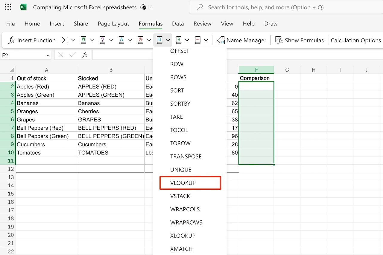
2. Go to Formulas > Lookup & Reference.

   

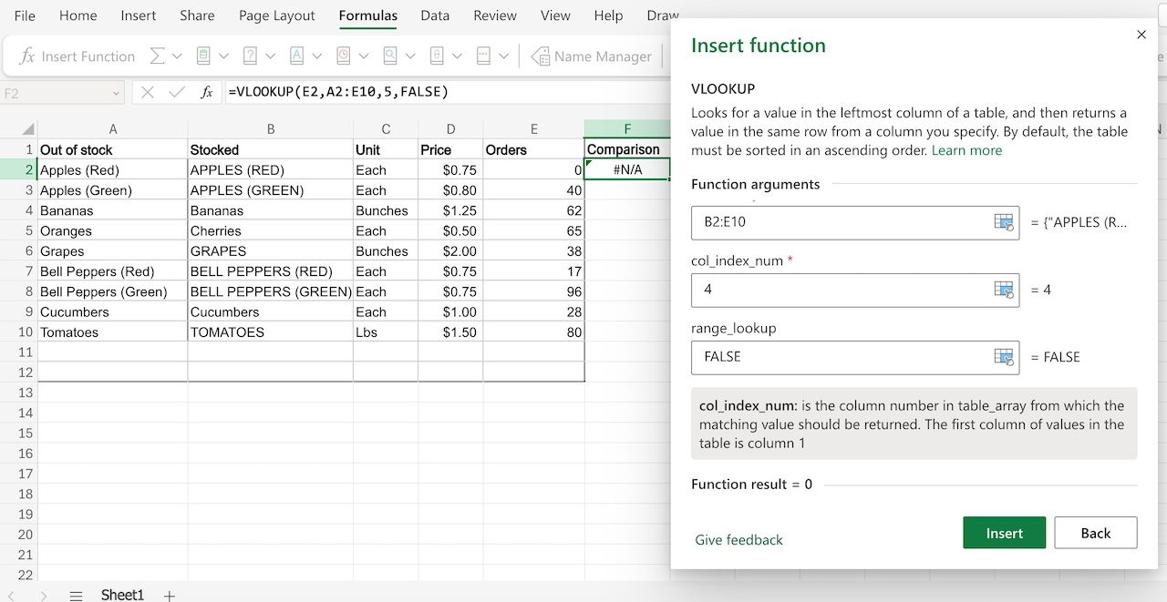
3. Select a cell containing the value you’re checking. For example, Apples.
4. Enter your table array. It’s the range of cells containing the data you want to search through. For example, B2:E10.
5. Under col_index_num, enter the column number within your table_array range from which you want to retrieve the corresponding value. Let’s say your table array ranges from column D to Column G. If the data you want is in Column G, enter 4.
6. Under range_lookup, specify whether you want an exact match (FALSE) or an approximate match (TRUE or omitted).
7. Click Insert.

   

8. Drag the lower-right edge of the cell containing the result across the cells underneath it. This action applies the appropriate values to them.

Related

How to create, record, and run Excel macros

Use Excel to its fullest in a few simple steps

Protect your Excel spreadsheet comparisons

Microsoft Excel is a powerful tool for consolidating and managing vast datasets. If you’re logged in to your Microsoft account on numerous devices, lock your workbooks so that no one touches your data without permission. Unless someone has the password, workbooks remain encrypted. You can also restrict access to your spreadsheets to select people you trust.