Introduction
When I started my deep learning journey, one of the first things I learned was image classification. It’s such a fascinating part of the computer vision fraternity and I was completely immersed in it! But I have a curious mind and once I had a handle on image classification, I wondered if I could transfer that learning to videos.
Was there a way to build a model that automatically identified specific people in a given video at a particular time interval? Turns out, there was and I’m excited to share my approach with you!
Source: Coastline Automation
Now to give you some context on the problem we’ll be solving, keep in mind that screen time is extremely important for an actor. It is directly related to the money he/she gets. Just to give you a sense of this commission, did you know that Robert Downey Jr. Downey picked up $10 million for just 15 minutes of screen time in “Spider-Man Homecoming”? Incredible.
How cool would it be if we could take any video and calculate the screen time of any actor present in it?
In this article, I will help you understand how to use deep learning on video data. To do this, we will be working with videos from the popular TOM and JERRY cartoon series. The aim is to calculate the screen time of both TOM and JERRY in any given video.
Sounds interesting? Read on then!
Note: This article assumes you have a prior knowledge of image classification using deep learning. If not, I recommend going through this article which will help you get a grasp of the basics of deep learning and image classification.
Table of Contents
- Reading a video and extracting frames
- How to handle video files in Python
- Calculating the screen time – A simple Solution
- My learnings – what worked and what did not
Reading a video and extracting frames
Ever heard of a flip book? If you haven’t, you’re missing out! Check out the one below:
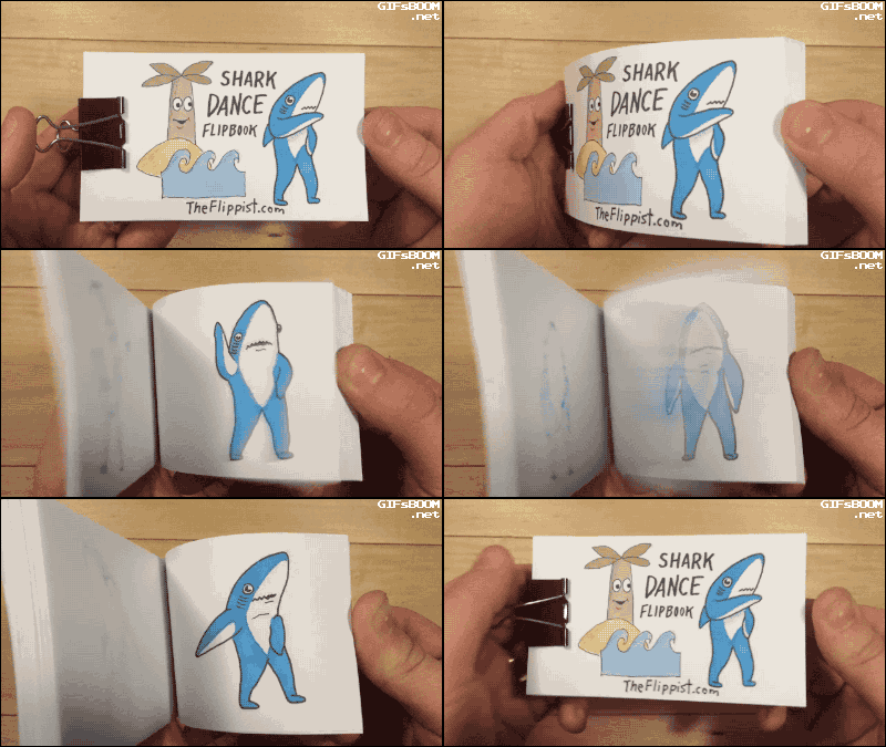
(Source: giphy.com)
We have a different image on each page of the book, and as we flip these pages, we get an animation of a shark dancing. You could even call it a kind of video. The visualization gets better the faster we flip the pages. In other words, this visual is a collection of different images arranged in a particular order.
Similarly, videos are nothing but a collection of a set of images. These images are called frames and can be combined to get the original video. So, a problem related to video data is not that different from an image classification or an object detection problem. There is just one extra step of extracting frames from the video.
Remember, our challenge here is to calculate the screen time of both Tom and Jerry from a given video. Let me first summarize the steps we will follow in this article to crack this problem:
- Import and read the video, extract frames from it, and save them as images
- Label a few images for training the model (Don’t worry, I have done it for you)
- Build our model on training data
- Make predictions for the remaining images
- Calculate the screen time of both TOM and JERRY
Believe me, just following these steps will help you in solving many such video related problems in deep learning. Time to get our Python hats on now, and dig into this challenge.
How to handle video files in Python
Let us start with importing all the necessary libraries. Go ahead and install the below libraries in case you haven’t already:
import cv2     # for capturing videos
import math   # for mathematical operations
import matplotlib.pyplot as plt    # for plotting the images
%matplotlib inline
import pandas as pd
from keras.preprocessing import image   # for preprocessing the images
import numpy as np    # for mathematical operations
from keras.utils import np_utils
from skimage.transform import resize   # for resizing images
Step – 1: Read the video, extract frames from it and save them as images
Now we will load the video and convert it into frames. You can download the video used for this example from this link. We will first capture the video from the given directory using the VideoCapture() function, and then we’ll extract frames from the video and save them as an image using the imwrite() function. Let’s code it:
Python Code:
Once this process is complete, ‘Done!’ will be printed on the screen as confirmation that the frames have been created.
Let us try to visualize an image (frame). We will first read the image using the imread() function of matplotlib, and then plot it using the imshow() function.
img = plt.imread('frame0.jpg')   # reading image using its name
plt.imshow(img)
Getting excited, yet?
This is the first frame from the video. We have extracted one frame for each second, from the entire duration of the video. Since the duration of the video is 4:58 minutes (298 seconds), we now have 298 images in total.
Our task is to identify which image has TOM, and which image has JERRY. If our extracted images would have been similar to the ones present in the popular Imagenet dataset, this challenge could have been a breeze. How? We could simply have used models pre-trained on that Imagenet data and achieved a high accuracy score! But then where’s the fun in that?
We have cartoon images so it’ll be very difficult (if not impossible) for any pre-trained model to identify TOM and JERRY in a given video.
Step – 2: Label a few images for training the model
So how do we go about handling this? A possible solution is to manually give labels to a few of the images and train the model on them. Once the model has learned the patterns, we can use it to make predictions on a previously unseen set of images.
Keep in mind that there could be frames when neither TOM nor JERRY are present. So, we will treat it as a multi-class classification problem. The classes which I have defined are:
- 0 – neither JERRY nor TOM
- 1 – for JERRY
- 2 – for TOM
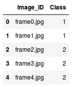
Don’t worry, I have labelled all the images so you don’t have to! Go ahead and download the mapping.csv file which contains each image name and their corresponding class (0 or 1 or 2).
data = pd.read_csv('mapping.csv')     # reading the csv file
data.head()      # printing first five rows of the file
The mapping file contains two columns:
- Image_ID: Contains the name of each image
- Class: Contains corresponding class for each image
Our next step is to read the images which we will do based on their names, aka, the Image_ID column.
X = [ ]     # creating an empty array
for img_name in data.Image_ID:
    img = plt.imread('' + img_name)
    X.append(img)  # storing each image in array X
X = np.array(X)    # converting list to array
Tada! We now have the images with us. Remember, we need two things to train our model:
- Training images, and
- Their corresponding class
Since there are three classes, we will one hot encode them using the to_categorical() function of keras.utils.
y = data.Class
dummy_y = np_utils.to_categorical(y)    # one hot encoding Classes
We will be using a VGG16 pretrained model which takes an input image of shape (224 X 224 X 3). Since our images are in a different size, we need to reshape all of them. We will use the resize() function of skimage.transform to do this.
image = []
for i in range(0,X.shape[0]):
    a = resize(X[i], preserve_range=True, output_shape=(224,224)).astype(int)      # reshaping to 224*224*3
    image.append(a)
X = np.array(image)
All the images have been reshaped to 224 X 224 X 3. But before passing any input to the model, we must preprocess it as per the model’s requirement. Otherwise, the model will not perform well enough. Use the preprocess_input() function of keras.applications.vgg16 to perform this step.
from keras.applications.vgg16 import preprocess_input
X = preprocess_input(X, mode='tf')      # preprocessing the input data
We also need a validation set to check the performance of the model on unseen images. We will make use of the train_test_split() function of the sklearn.model_selection module to randomly divide images into training and validation set.
from sklearn.model_selection import train_test_split
X_train, X_valid, y_train, y_valid = train_test_split(X, dummy_y, test_size=0.3, random_state=42)    # preparing the validation set
Step 3: Building the model
The next step is to build our model. As mentioned, we shall be using the VGG16 pretrained model for this task. Let us first import the required libraries to build the model:
from keras.models import Sequential
from keras.applications.vgg16 import VGG16
from keras.layers import Dense, InputLayer, Dropout
We will now load the VGG16 pretrained model and store it as base_model:
base_model = VGG16(weights='imagenet', include_top=False, input_shape=(224, 224, 3)) # include_top=False to remove the top layer
We will make predictions using this model for X_train and X_valid, get the features, and then use those features to retrain the model.
X_train = base_model.predict(X_train)
X_valid = base_model.predict(X_valid)
X_train.shape, X_valid.shape
The shape of X_train and X_valid is (208, 7, 7, 512), (90, 7, 7, 512) respectively. In order to pass it to our neural network, we have to reshape it to 1-D.
X_train = X_train.reshape(208, 7*7*512)      # converting to 1-D
X_valid = X_valid.reshape(90, 7*7*512)
We will now preprocess the images and make them zero-centered which helps the model to converge faster.
train = X_train/X_train.max()      # centering the data
X_valid = X_valid/X_train.max()
Finally, we will build our model. This step can be divided into 3 sub-steps:
- Building the model
- Compiling the model
- Training the model
# i. Building the model
model = Sequential()
model.add(InputLayer((7*7*512,)))    # input layer
model.add(Dense(units=1024, activation='sigmoid')) # hidden layer
model.add(Dense(3, activation='softmax'))    # output layer
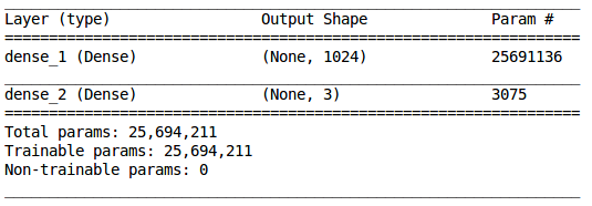
Let’s check the summary of the model using the summary() function:
model.summary()
We have a hidden layer with 1,024 neurons and an output layer with 3 neurons (since we have 3 classes to predict). Now we will compile our model:
# ii. Compiling the model
model.compile(loss='categorical_crossentropy', optimizer='adam', metrics=['accuracy'])
In the final step, we will fit the model and simultaneously also check its performance on the unseen images, i.e., validation images:
# iii. Training the model
model.fit(train, y_train, epochs=100, validation_data=(X_valid, y_valid))
We can see it is performing really well on the training as well as the validation images. We got an accuracy of around 85% on unseen images. And this is how we train a model on video data to get predictions for each frame.
In the next section, we will try to calculate the screen time of TOM and JERRY in a new video.
Calculating the screen time – A simple solution
First, download the video we’ll be using in this section from here. Once done, go ahead and load the video and extract frames from it. We will follow the same steps as we did above:
count = 0
videoFile = "Tom and Jerry 3.mp4"
cap = cv2.VideoCapture(videoFile)
frameRate = cap.get(5) #frame rate
x=1
while(cap.isOpened()):
    frameId = cap.get(1) #current frame number
    ret, frame = cap.read()
    if (ret != True):
        break
    if (frameId % math.floor(frameRate) == 0):
        filename ="test%d.jpg" % count;count+=1
        cv2.imwrite(filename, frame)
cap.release()
print ("Done!")
Done!
After extracting the frames from the new video, we will now load the test.csv file which contains the names of each extracted frame. Download the test.csv file and load it:
test = pd.read_csv('test.csv')
Next, we will import the images for testing and then reshape them as per the requirements of the aforementioned pretrained model:
test_image = []
for img_name in test.Image_ID:
    img = plt.imread('' + img_name)
    test_image.append(img)
test_img = np.array(test_image)
test_image = []
for i in range(0,test_img.shape[0]):
    a = resize(test_img[i], preserve_range=True, output_shape=(224,224)).astype(int)
    test_image.append(a)
test_image = np.array(test_image)
We need to make changes to these images similar to the ones we did for the training images. We will preprocess the images, use the base_model.predict() function to extract features from these images using the VGG16 pretrained model, reshape these images to 1-D form, and make them zero-centered:
# preprocessing the images
test_image = preprocess_input(test_image, mode='tf')

# extracting features from the images using pretrained model
test_image = base_model.predict(test_image)

# converting the images to 1-D form
test_image = test_image.reshape(186, 7*7*512)

# zero centered images
test_image = test_image/test_image.max()
Since we have trained the model previously, we will make use of that model to make prediction for these images.
Step – 4: Make predictions for the remaining images
predictions = model.predict_classes(test_image)
Step – 5 Calculate the screen time of both TOM and JERRY
Recall that Class ‘1’ represents the presence of JERRY, while Class ‘2’ represents the presence of TOM. We shall make use of the above predictions to calculate the screen time of both these legendary characters:
print("The screen time of JERRY is", predictions[predictions==1].shape[0], "seconds")
print("The screen time of TOM is", predictions[predictions==2].shape[0], "seconds")
And there you go! We have the total screen time of both TOM and JERRY in the given video.
My learnings – what worked and what did not
I tried and tested many things for this challenge – some worked exceedingly well, while some ended up flat. In this section, I will elaborate a bit on some of the difficulties I faced, and then how I tackled them. After that, I have provided the entire code for the final model which gave me the best accuracy.
First, I tried using the pretrained model without removing the top layer. The results were not satisfactory. The possible reason could be that these are the cartoon images and our pretrained model was trained on actual images and hence it was not able to classify these cartoon images. To tackle this problem, i retrained the pretrain model using few labelled images and the results were better from the previous results.
Even after training on the labelled images, the accuracy was not satisfactory. The model was not able to perform well on the training images itself. So, i tried to increase the number of layers. Increasing the number of layers proved to be a good solution to increase the training accuracy but there was no sync between training and validation accuracy. The model was overfitting and its performance on the unseen data was not satisfactory. So I added a Dropout layer after every Dense layer and then there was good sync between training and validation accuracy.
I noticed that the classes are imbalanced. TOM had more screen time so the predictions were dominated by it and most of the frames were predicted as TOM. To overcome this and make the classes balanced, i used compute_class_weight() function of sklearn.utils.class_weight module. It assigned higher weights to the classes with lower value counts as compared to the classes with higher value counts.
I also used Model Checkpointing to save the best model, i.e. the model which produced lowest validation loss and then used that model to make the final predictions. I will summarize all the above mentioned steps and will give the final code now. The actual classes for the testing images can be found in testing.csv file.
import cv2
import math
import matplotlib.pyplot as plt
import pandas as pd
%matplotlib inline
from keras.preprocessing import image
import numpy as np
from skimage.transform import resize
count = 0
videoFile = "Tom and jerry.mp4"
cap = cv2.VideoCapture(videoFile)
frameRate = cap.get(5) #frame rate
x=1
while(cap.isOpened()):
    frameId = cap.get(1) #current frame number
    ret, frame = cap.read()
    if (ret != True):
        break
    if (frameId % math.floor(frameRate) == 0):
        filename ="frame%d.jpg" % count;count+=1
        cv2.imwrite(filename, frame)
cap.release()
print ("Done!")
Done!
count = 0
videoFile = "Tom and Jerry 3.mp4"
cap = cv2.VideoCapture(videoFile)
frameRate = cap.get(5) #frame rate
x=1
while(cap.isOpened()):
    frameId = cap.get(1) #current frame number
    ret, frame = cap.read()
    if (ret != True):
        break
    if (frameId % math.floor(frameRate) == 0):
        filename ="test%d.jpg" % count;count+=1
        cv2.imwrite(filename, frame)
cap.release()
print ("Done!")
Done!
data = pd.read_csv('mapping.csv')
test = pd.read_csv('testing.csv')
X = []
for img_name in data.Image_ID:
    img = plt.imread('' + img_name)
    X.append(img)
X = np.array(X)
test_image = []
for img_name in test.Image_ID:
    img = plt.imread('' + img_name)
    test_image.append(img)
test_img = np.array(test_image)
from keras.utils import np_utils
train_y = np_utils.to_categorical(data.Class)
test_y = np_utils.to_categorical(test.Class)
image = []
for i in range(0,X.shape[0]):
    a = resize(X[i], preserve_range=True, output_shape=(224,224,3)).astype(int)
    image.append(a)
X = np.array(image)
test_image = []
for i in range(0,test_img.shape[0]):
    a = resize(test_img[i], preserve_range=True, output_shape=(224,224)).astype(int)
    test_image.append(a)
test_image = np.array(test_image)
from keras.applications.vgg16 import preprocess_input
X = preprocess_input(X, mode='tf')
test_image = preprocess_input(test_image, mode='tf')
from sklearn.model_selection import train_test_split
X_train, X_valid, y_train, y_valid = train_test_split(X, train_y, test_size=0.3, random_state=42)
from keras.models import Sequential
from keras.applications.vgg16 import VGG16
from keras.layers import Dense, InputLayer, Dropout
base_model = VGG16(weights='imagenet', include_top=False, input_shape=(224, 224, 3))
X_train = base_model.predict(X_train)
X_valid = base_model.predict(X_valid)
test_image = base_model.predict(test_image)
X_train = X_train.reshape(208, 7*7*512)
X_valid = X_valid.reshape(90, 7*7*512)
test_image = test_image.reshape(186, 7*7*512)
train = X_train/X_train.max()
X_valid = X_valid/X_train.max()
test_image = test_image/test_image.max()
model = Sequential()
model.add(InputLayer((7*7*512,)))    # input layer
model.add(Dense(units=1024, activation='sigmoid'))   # hidden layer
model.add(Dropout(0.5))      # adding dropout
model.add(Dense(units=512, activation='sigmoid'))    # hidden layer
model.add(Dropout(0.5))      # adding dropout
model.add(Dense(units=256, activation='sigmoid'))    # hidden layer
model.add(Dropout(0.5))      # adding dropout
model.add(Dense(3, activation='softmax'))            # output layer
model.compile(loss='categorical_crossentropy', optimizer='adam', metrics=['accuracy'])
from sklearn.utils.class_weight import compute_class_weight, compute_sample_weight
class_weights = compute_class_weight('balanced',np.unique(data.Class), data.Class)  # computing weights of different classes
from keras.callbacks import ModelCheckpoint
filepath="weights.best.hdf5"
checkpoint = ModelCheckpoint(filepath, monitor='val_loss', verbose=1, save_best_only=True, mode='min')
callbacks_list = [checkpoint]      # model check pointing based on validation loss
model.fit(train, y_train, epochs=100, validation_data=(X_valid, y_valid), class_weight=class_weights, callbacks=callbacks_list)
model.load_weights("weights.best.hdf5")
model.compile(loss='categorical_crossentropy', optimizer='adam', metrics=['accuracy'])
scores = model.evaluate(test_image, test_y)
print("%s: %.2f%%" % (model.metrics_names[1], scores[1]*100))
Conclusion
We got an accuracy of around 88% on the validation data and 64% on the test data using this model.
One possible reason for getting a low accuracy on test data could be a lack of training data. As the model does not have much knowledge of cartoon images like TOM and JERRY, we must feed it more images during the training process. My advice would be to extract more frames from different TOM and JERRY videos, label them accordingly, and use them for training the model. Once the model has seen a plethora of images of these two characters, there’s a good chance it will lead to a better classification result.
Such models can help us in various fields:
- We can calculate the screen time of a particular actor in a movie
- Calculate the screen time of your favorite superhero, etc.
These are just a few examples where this technique can be used. You can come up with many more such applications on your own! Feel free to share your thoughts and feedback in the comments section below.


