Introduction
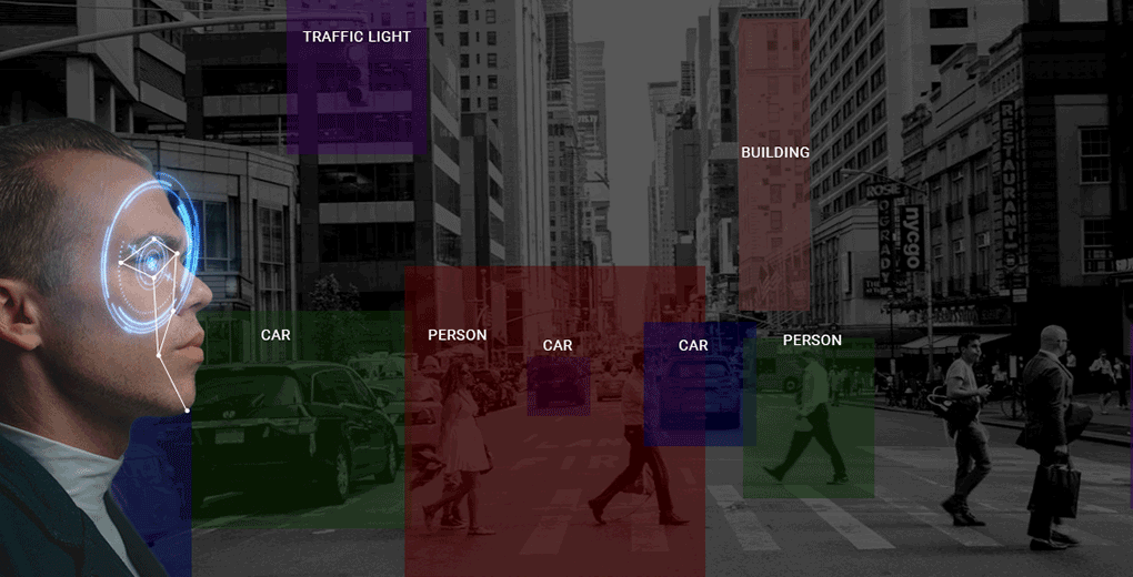
Computer vision is among the hottest fields in any industry right now. It is thriving thanks to the rapid advances in technology and research. But it can be a daunting space for newcomers. There are some common challenges data scientists face when transitioning into computer vision, including:
- How do we clean image datasets? Images come in different shapes and sizes
- The ever-present problem of acquiring data. Should we collect more images before building our computer vision model?
- Is learning deep learning compulsory for building computer vision models? Can we not use machine learning techniques?
- Can we build a computer vsiion model on our own machine? Not everyone has access to GPUs and TPUs!
I certainly faced most of these challenges and I’m sure most of you must have as well. These are the right questions to ask as a beginner in computer vision – so good news! You are in the right place.
In this article, we will answer most of these questions through the awesome OpenCV library. It stands out like a beacon for computer vision tasks and is easily the most popular CV library around.
But OpenCV comes with a caveat – it can be a little tough to navigate for newcomers. There are a plethora of functions available inside OpenCV, but it can become daunting to:
- Understand the wide variety of functions available
- Gauge which function to use for your particular problem
I personally believe learning how to navigate OpenCV is a must for any computer vision enthusiast. Hence, I decided to write this article detailing the different (common) functions inside OpenCV, their applications, and how you can get started with each one. There is Python code in this article so be ready with your Notebooks!
Note: This article assumes you are familiar with computer vision terminology. If you’re new to the topic, check out the below resources:
- Deep Learning for Computer Vision – Introduction to Convolution Neural Networks (CNNs)
- Build your First Image Classification Model in just 10 Minutes!
- Computer Vision using Deep Learning Course
Table of Contents
- What is Computer Vision?
- Why use OpenCV for Computer Vision Tasks?
- Reading, Writing and Displaying Images
- Changing Color Spaces
- Resizing Images
- Image Rotation
- Image Translation
- Simple Image Thresholding
- Adaptive Thresholding
- Image Segmentation (Watershed Algorithm)
- Bitwise Operations
- Edge Detection
- Image Filtering
- Image Contours
- Scale Invariant Feature Transform (SIFT)
- Speeded-Up Robust Features (SURF)
- Feature Matching
- Face Detection
What is Computer Vision?
Let me quickly explain what computer vision is before we dive into OpenCV. It’s good to have an intuitive understanding of what we’ll be talking about through the rest of the article.
The ability to see and perceive the world comes naturally to us humans. It’s second nature for us to gather information from our surroundings through the gift of vision and perception.
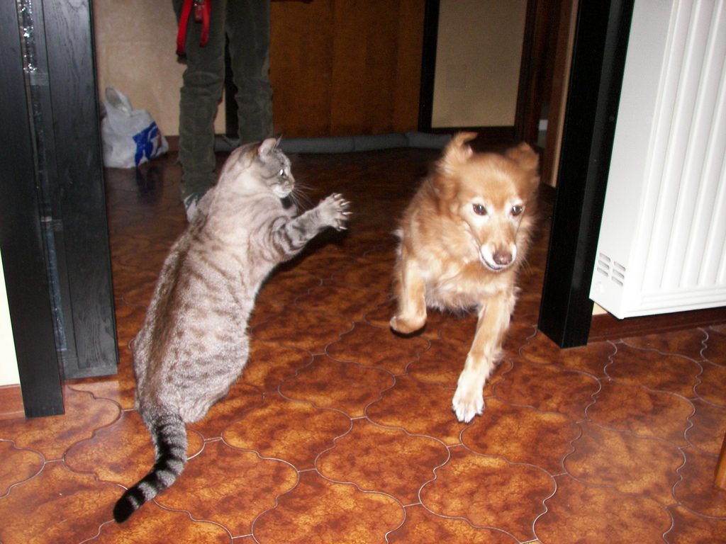
Take a quick look at the above image. It takes us less than a second to figure out there’s a cat, a dog and a pair of human legs. When it comes to machines, this learning process becomes complicated. The process of parsing through an image and detecting objects involves multiple and complex steps, including feature extraction (edges detection, shapes, etc), feature classification, etc.
Computer Vision is a field of deep learning that enables machines to see, identify and process images like humans.
Computer vision is one of the hottest fields in the industry right now. You can expect plenty of job openings to come up in the next 2-4 years. The question then is – are you ready to take advantage of these opportunities?
Take a moment to ponder this – which applications or products come to your mind when you think of computer vision? The list is HUGE. We use some of them everyday! Features like unlocking our phones using face recognition, our smartphone cameras, self-driving cars – computer vision is everywhere.
Why use OpenCV for Computer Vision Tasks?
OpenCV, or Open Source Computer Vision library, started out as a research project at Intel. It’s currently the largest computer vision library in terms of the sheer number of functions it holds.
OpenCV contains implementations of more than 2500 algorithms! It is freely available for commercial as well as academic purposes. And the joy doesn’t end there! The library has interfaces for multiple languages, including Python, Java, and C++.
The first OpenCV version, 1.0, was released in 2006 and the OpenCV community has grown leaps and bounds since then.
Now, let’s turn our attention to the idea behind this article – the plethora of functions OpenCV offers! We will be looking at OpenCV from the perspective of a data scientist and learning about some functions that make the task of developing and understanding computer vision models easier.
Reading, Writing and Displaying Images
Machines see and process everything using numbers, including images and text. How do you convert images to numbers – I can hear you wondering. Two words – pixel values:
Every number represents the pixel intensity at that particular location. In the above image, I have shown the pixel values for a grayscale image where every pixel contains only one value i.e. the intensity of the black color at that location.
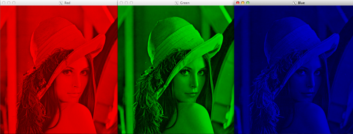
Note that color images will have multiple values for a single pixel. These values represent the intensity of respective channels – Red, Green and Blue channels for RGB images, for instance.
Reading and writing images is essential to any computer vision project. And the OpenCV library makes this function a whole lot easier.
Now, let’s see how to import an image into our machine using OpenCV. Download the image from here.
Python Code:
By default, the imread function reads images in the BGR (Blue-Green-Red) format. We can read images in different formats using extra flags in the imread function:
- cv2.IMREAD_COLOR: Default flag for loading a color image
- cv2.IMREAD_GRAYSCALE: Loads images in grayscale format
- cv2.IMREAD_UNCHANGED: Loads images in their given format, including the alpha channel. Alpha channel stores the transparency information – the higher the value of alpha channel, the more opaque is the pixel
Changing Color Spaces
A color space is a protocol for representing colors in a way that makes them easily reproducible. We know that grayscale images have single pixel values and color images contain 3 values for each pixel – the intensities of the Red, Green and Blue channels.
Most computer vision use cases process images in RGB format. However, applications like video compression and device independent storage – these are heavily dependent on other color spaces, like the Hue-Saturation-Value or HSV color space.
As you understand a RGB image consists of the color intensity of different color channels, i.e. the intensity and color information are mixed in RGB color space but in HSV color space the color and intensity information are separated from each other. This makes HSV color space more robust to lighting changes.
OpenCV reads a given image in the BGR format by default. So, you’ll need to change the color space of your image from BGR to RGB when reading images using OpenCV. Let’s see how to do that:
Resizing Images
Machine learning models work with a fixed sized input. The same idea applies to computer vision models as well. The images we use for training our model must be of the same size.
Now this might become problematic if we are creating our own dataset by scraping images from various sources. That’s where the function of resizing images comes to the fore.
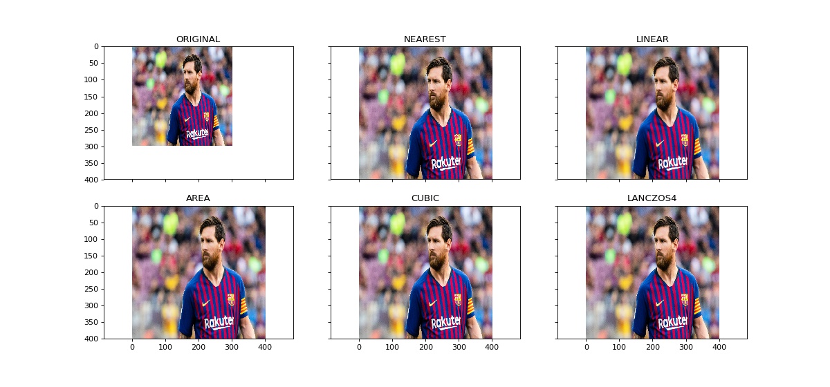
Images can be easily scaled up and down using OpenCV. This operation is useful for training deep learning models when we need to convert images to the model’s input shape. Different interpolation and downsampling methods are supported by OpenCV, which can be used by the following parameters:
- INTER_NEAREST: Nearest neighbor interpolation
- INTER_LINEAR: Bilinear interpolation
- INTER_AREA: Resampling using pixel area relation
- INTER_CUBIC: Bicubic interpolation over 4×4 pixel neighborhood
- INTER_LANCZOS4: Lanczos interpolation over 8×8 neighborhood
OpenCV’s resize function uses bilinear interpolation by default.
Image Rotation
“You need a large amount of data to train a deep learning model”. I’m sure you must have comes across this line of thought in form or another. It’s partially true – most deep learning algorithms are heavily dependent on the quality and quantity of the data.
But what if you do not have a large enough dataset? Not all of us can afford to manually collect and label images.
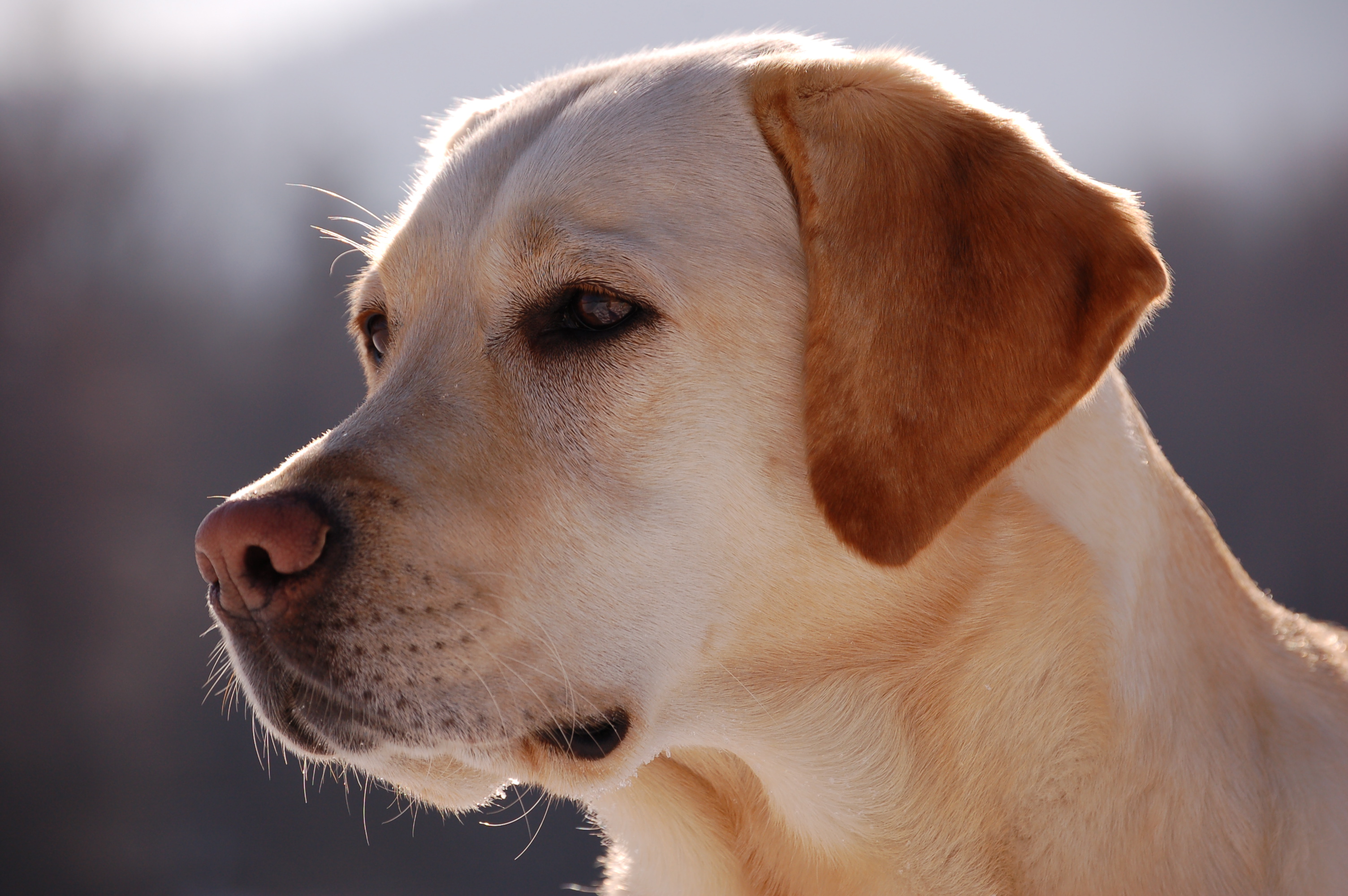
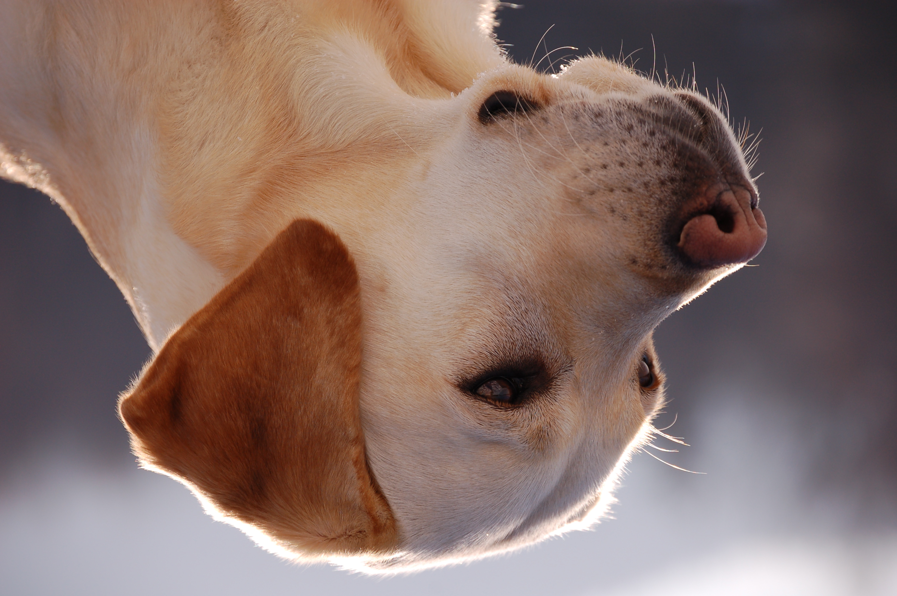
Suppose we are building an image classification model for identifying the animal present in an image. So, both the images shown below should be classified as ‘dog’:
But the model might find it difficult to classify the second image as a Dog if it was not trained on such images. So what should we do?
Let me introduce you to the technique of data augmentation. This method allows us to generate more samples for training our deep learning model. Data augmentation uses the available data samples to produce the new ones, by applying image operations like rotation, scaling, translation, etc. This makes our model robust to changes in input and leads to better generalization.
Rotation is one of the most used and easy to implement data augmentation techniques. As the name suggests, it involves rotating the image at an arbitrary angle and providing it the same label as the original image. Think of the times you have rotated images in your phone to achieve certain angles – that’s basically what this function does.
Image Translation
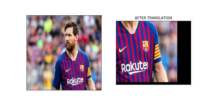
Image translation is a geometric transformation that maps the position of every object in the image to a new location in the final output image. After the translation operation, an object present at location (x,y) in the input image is shifted to a new position (X,Y):
X = x + dx
Y = y + dy
Here, dx and dy are the respective translations along different dimensions.
Image translation can be used to add shift invariance to the model, as by tranlation we can change the position of the object in the image give more variety to the model that leads to better generalizability which works in difficult conditions i.e. when the object is not perfectly aligned to the center of the image.
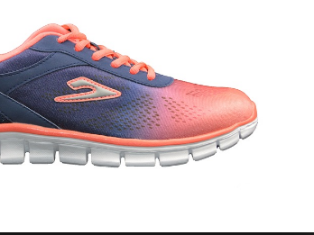
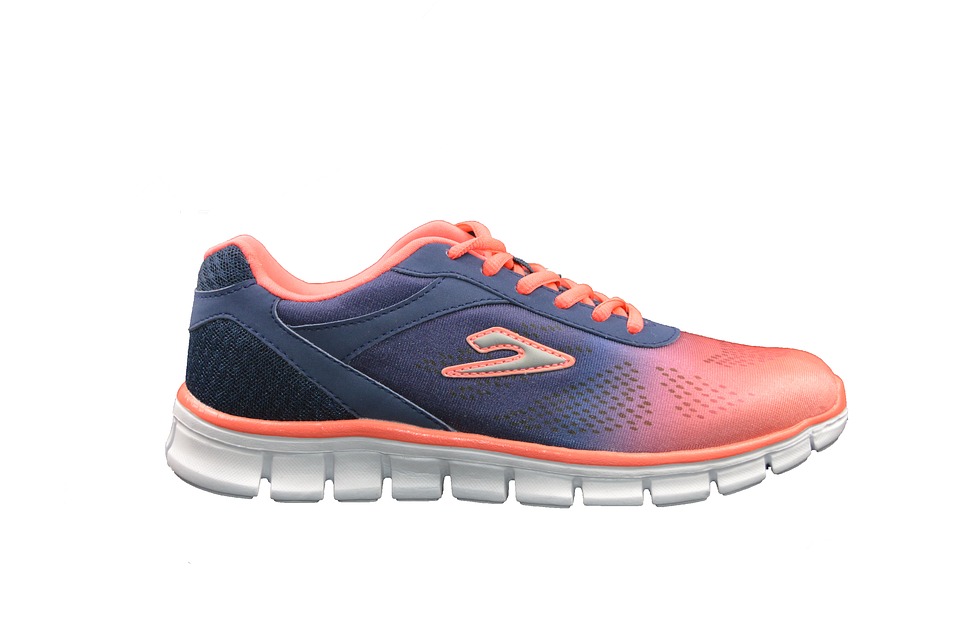
This augmentation technique can also help the model correctly classify images with partially visible objects. Take the below image for example. Even when the complete shoe is not present in the image, the model should be able to classify it as a Shoe.
This translation function is typically used in the image pre-processing stage. Check out the below code to see how it works in a practical scenario:
Simple Image Thresholding
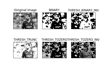
Thresholding is an image segmentation method. It compares pixel values with a threshold value and updates it accordingly. OpenCV supports multiple variations of thresholding. A simple thresholding function can be defined like this:
if Image(x,y) > threshold , Image(x,y) = 1
otherswise, Image(x,y) = 0
Thresholding can only be applied to grayscale images.
A simple application of image thresholding could be dividing the image into it’s foreground and background.
Adaptive Thresholding
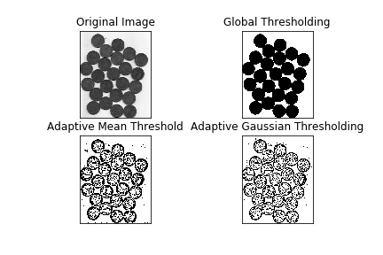
In case of adaptive thresholding, different threshold values are used for different parts of the image. This function gives better results for images with varying lighting conditions – hence the term “adaptive”.
Otsu’s binarization method finds an optimal threshold value for the whole image. It works well for bimodal images (images with 2 peaks in their histogram).
Image Segmentation (Watershed Algorithm)
Image segmentation is the task of classifying every pixel in the image to some class. For example, classifying every pixel as foreground or background. Image segmentation is important for extracting the relevant parts from an image.
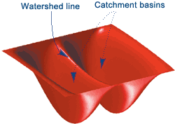
The watershed algorithm is a classic image segmentation algorithm. It considers the pixel values in an image as topography. For finding the object boundaries, it takes initial markers as input. The algorithm then starts flooding the basin from the markers till the markers meet at the object boundaries.
Image Source :- Mathworks
Let’s say we have a topography with multiple basins. Now, if we fill different basins with water of different color, then the intersection of different colors will give us the object boundaries. This is the intuition behind the watershed algorithm.
Bitwise Operations
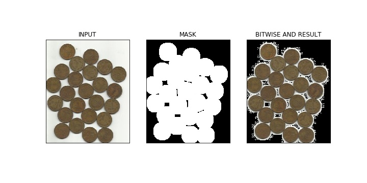
Bitwise operations include AND, OR, NOT and XOR. You might remember them from your programming class! In computer vision, these operations are very useful when we have a mask image and want to apply that mask over another image to extract the region of interest.
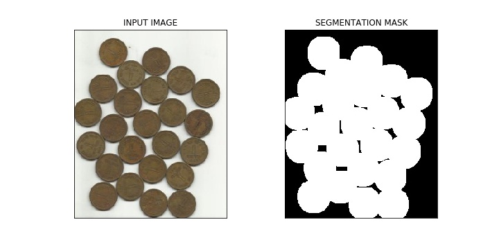
In the above figure, we can see an input image and its segmentation mask calculated using the Watershed algorithm. Further, we have applied the bitwise ‘AND’ operation to remove the background from the image and extract relevant portions from the image. Pretty awesome stuff!
Edge Detection
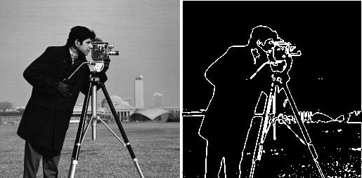
Edges are the points in an image where the image brightness changes sharply or has discontinuities. Such discontinuities generally correspond to:
- Discontinuities in depth
- Discontinuities in surface orientation
- Changes in material properties
- Variations in scene illumination
Edges are very useful features of an image that can be used for different applications like classification of objects in the image and localization. Even deep learning models calculate edge features to extract information about the objects present in image.
Edges are different from contours as they are not related to objects rather they signify the changes in pixel values of an image. Edge detection can be used for image segmentation and even for image sharpening.
Image Filtering
In image filtering, a pixel value is updated using its neighbouring values. But how are these values updated in the first place?
Well, there are multiple ways of updating pixel values, such as selecting the maximum value from neighbours, using the average of neighbours, etc. Each method has it’s own uses. For example, averaging the pixel values in a neighbourhood is used for image blurring.
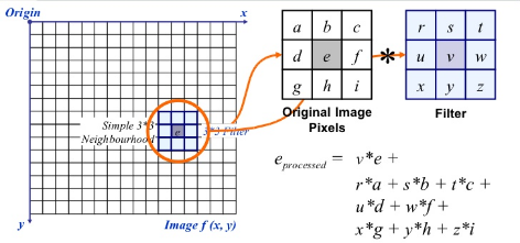
Image Source:- Google
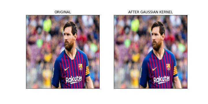
Gaussian filtering is also used for image blurring that gives different weights to the neighbouring pixels based on their distance from the pixel under consideration.
For image filtering, we use kernels. Kernels are matrices of numbers of different shapes like 3 x 3, 5 x 5, etc. A kernel is used to calculate the dot product with a part of the image. When calculating the new value of a pixel, the kernel center is overlapped with the pixel. The neighbouring pixel values are multiplied with the corresponding values in the kernel. The calculated value is assigned to the pixel coinciding with the center of the kernel.
In the above output, the image on the right shows the result of applying Gaussian kernels on an input image. We can see that the edges of the original image are suppressed. The Gaussian kernel with different values of sigma is used extensively to calculate the Difference of Gaussian for our image. This is an important step in the feature extraction process because it reduces the noise present in the image.
Image Contours
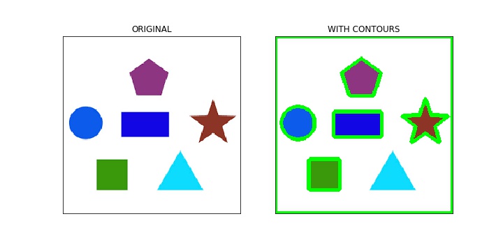
A contour is a closed curve of points or line segments that represents the boundaries of an object in the image. Contours are essentially the shapes of objects in an image.
Unlike edges, contours are not part of an image. Instead, they are an abstract collection of points and line segments corresponding to the shapes of the object(s) in the image.
We can use contours to count the number of objects in an image, categorize objects on the basis of their shapes, or select objects of particular shapes from the image.
Scale Invariant Feature Transform (SIFT)
Keypoints is a concept you should be aware of when working with images. These are basically the points of interest in an image. Keypoints are analogous to the features of a given image.
They are locations that define what is interesting in the image. Keypoints are important, because no matter how the image is modified (rotation, shrinking, expanding, distortion), we will always find the same keypoints for the image.
Scale Invariant Feature Transform (SIFT) is a very popular keypoint detection algorithm. It consists of the following steps:
- Scale-space extrema detection
- Keypoint localization
- Orientation assignment
- Keypoint descriptor
- Keypoint matching
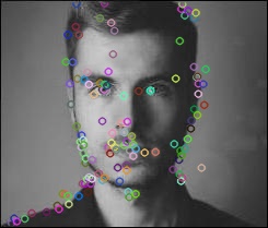
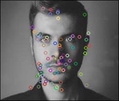
Features extracted from SIFT can be used for applications like image stitching, object detection, etc. The below code and output show the keypoints and their orientation calculated using SIFT.
Speeded-Up Robust Features (SURF)
Speeded-Up Robust Features (SURF) is an enhanced version of SIFT. It works much faster and is more robust to image transformations. In SIFT, the scale space is approximated using Laplacian of Gaussian. Wait – that sounds too complex. What is Laplacian of Gaussian?
Laplacian is a kernel used for calculating the edges in an image. The Laplacian kernel works by approximating a second derivative of the image. Hence, it is very sensitive to noise. We generally apply the Gaussian kernel to the image before Laplacian kernel thus giving it the name Laplacian of Gaussian.
In SURF, the Laplacian of Gaussian is calculated using a box filter (kernel). The convolution with box filter can be done in parallel for different scales which is the underlying reason for the enhanced speed of SURF (compared to SIFT). There are other neat improvements like this in SURF – I suggest going through the research paper to understand this in-depth.
Feature Matching
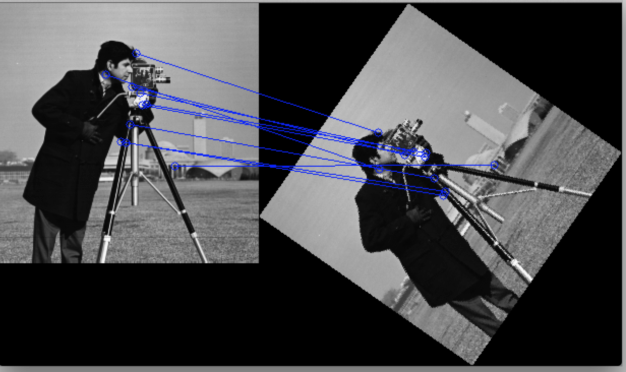
The features extracted from different images using SIFT or SURF can be matched to find similar objects/patterns present in different images. The OpenCV library supports multiple feature-matching algorithms, like brute force matching, knn feature matching, among others.
In the above image, we can see that the keypoints extracted from the original image (on the left) are matched to keypoints of its rotated version. This is because the features were extracted using SIFT, which is invariant to such transformations.
Face Detection
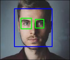
OpenCV supports haar cascade based object detection. Haar cascades are machine learning based classifiers that calculate different features like edges, lines, etc in the image. Then, these classifiers train using multiple positive and negative samples.
Trained classifiers for different objects like faces,eyes etc are available in the OpenCV Github repo , you can also train your own haar cascade for any object.
Make sure you go through the below excellent article that teaches you how to build a face detection model from video using OpenCV:
And if you’re looking to learn the face detection concept from scratch, then this article should be of interest.
End Notes
OpenCV is truly an all emcompassing library for computer vision tasks. I hope you tried out all the above codes on your machine – the best way to learn computer vision is by applying it on your own. I encourage you to build your own applications and experiment with OpenCV as much as you can.
OpenCV is continually adding new modules for latest algorithms from Machine learning, do check out their Github repository and get familiar with implementation. You can even contribute to the library which is a great way to learn and interact with the community.
Are you a computer vision newcomer? Start your journey here:


