Overview
- Activation function is one of the building blocks on Neural Network
- Learn about the different activation functions in deep learning & types of activation function
- Code activation functions in python and visualize results in live coding window
This article was originally published in October 2017 and updated in January 2020 with three new activation functions and python codes.
Introduction
The Internet provides access to plethora of information today. Whatever we need is just a Google (search) away. However, when we have so much information, the challenge is to segregate between relevant and irrelevant information.
When our brain is fed with a lot of information simultaneously, it tries hard to understand and classify the information into “useful” and “not-so-useful” information. We need a similar mechanism for classifying incoming information as “useful” or “less-useful” in case of Neural Networks.

This is important in the way a network learns because not all the information is equally useful. Some of it is just noise. This is where activation functions come into picture. The activation functions help the network use the important information and suppress the irrelevant data points.
Let us go through these activation functions, learn how they work and figure out which activation functions fits well into what kind of problem statement.
Table of contents
Brief overview of neural networks
Before I delve into the details of activation functions, let us quickly go through the concept of neural networks and how they work. A neural network is a very powerful machine learning mechanism which basically mimics how a human brain learns.
The brain receives the stimulus from the outside world, does the processing on the input, and then generates the output. As the task gets complicated, multiple neurons form a complex network, passing information among themselves.
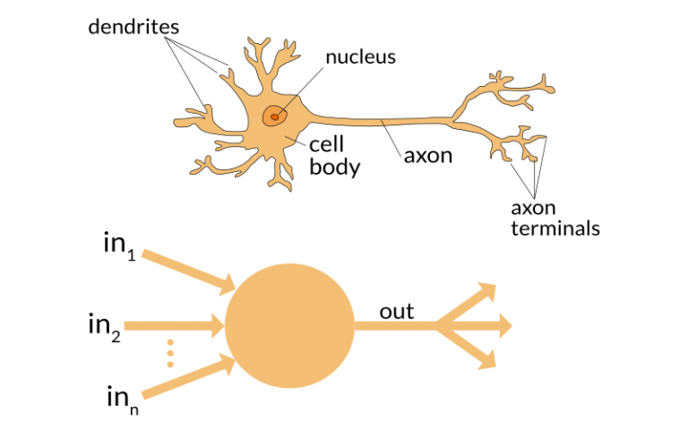
An Artificial Neural Network tries to mimic a similar behavior. The network you see below is a neural network made of interconnected neurons. Each neuron is characterized by its weight, bias and activation function.
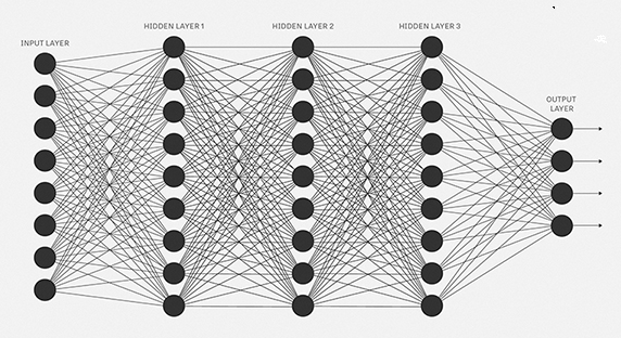
The input is fed to the input layer, the neurons perform a linear transformation on this input using the weights and biases.
x = (weight * input) + bias
Post that, an activation function is applied on the above result.

Finally, the output from the activation function moves to the next hidden layer and the same process is repeated. This forward movement of information is known as the forward propagation.
What if the output generated is far away from the actual value? Using the output from the forward propagation, error is calculated. Based on this error value, the weights and biases of the neurons are updated. This process is known as back-propagation.
Note: To understand forward and backward propagation in detail, you can go through the following article-
Can we do without an activation function?
We understand that using an activation function introduces an additional step at each layer during the forward propagation. Now the question is – if the activation function increases the complexity so much, can we do without an activation function?
Imagine a neural network without the activation functions. In that case, every neuron will only be performing a linear transformation on the inputs using the weights and biases. Although linear transformations make the neural network simpler, but this network would be less powerful and will not be able to learn the complex patterns from the data.
A neural network without an activation function is essentially just a linear regression model.
Thus we use a non linear transformation to the inputs of the neuron and this non-linearity in the network is introduced by an activation function.
In the next section we will look at the different types of Activation Functions, their mathematical equations, graphical representation and python codes.
Popular types of activation functions and when to use them
1. Binary Step Function
The first thing that comes to our mind when we have an activation function would be a threshold based classifier i.e. whether or not the neuron should be activated based on the value from the linear transformation.
In other words, if the input to the activation function is greater than a threshold, then the neuron is activated, else it is deactivated, i.e. its output is not considered for the next hidden layer. Let us look at it mathematically-
f(x) = 1, x>=0
     = 0, x<0
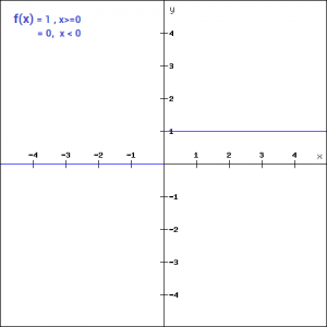
This is the simplest activation function, which can be implemented with a single if-else condition in python
def binary_step(x):
    if x<0:
        return 0
    else:
        return 1
binary_step(5), binary_step(-1)
Output:
(1,0)
The binary step function can be used as an activation function while creating a binary classifier. As you can imagine, this function will not be useful when there are multiple classes in the target variable. That is one of the limitations of binary step function.
Moreover, the gradient of the step function is zero which causes a hindrance in the back propagation process. That is, if you calculate the derivative of f(x) with respect to x, it comes out to be 0.
f'(x) = 0, for all x
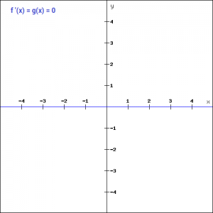
Gradients are calculated to update the weights and biases during the backprop process. Since the gradient of the function is zero, the weights and biases don’t update.
2. Linear Function
We saw the problem with the step function, the gradient of the function became zero. This is because there is no component of x in the binary step function. Instead of a binary function, we can use a linear function. We can define the function as-
f(x)=ax
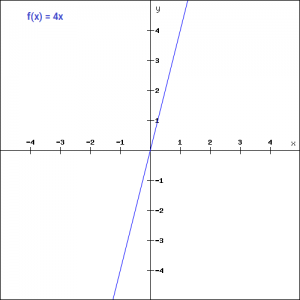
Here the activation is proportional to the input.The variable ‘a’ in this case can be any constant value. Let’s quickly define the function in python:
def linear_function(x):
    return 4*x
linear_function(4), linear_function(-2)
Output:
(16, -8)
What do you think will be the derivative is this case? When we differentiate the function with respect to x, the result is the coefficient of x, which is a constant.
f'(x) = a
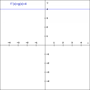
Although the gradient here does not become zero, but it is a constant which does not depend upon the input value x at all. This implies that the weights and biases will be updated during the backpropagation process but the updating factor would be the same.
In this scenario, the neural network will not really improve the error since the gradient is the same for every iteration. The network will not be able to train well and capture the complex patterns from the data. Hence, linear function might be ideal for simple tasks where interpretability is highly desired.
3. Sigmoid
The next activation function that we are going to look at is the Sigmoid function. It is one of the most widely used non-linear activation function. Sigmoid transforms the values between the range 0 and 1. Here is the mathematical expression for sigmoid-
f(x) = 1/(1+e^-x)
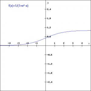
A noteworthy point here is that unlike the binary step and linear functions, sigmoid is a non-linear function. This essentially means -when I have multiple neurons having sigmoid function as their activation function,the output is non linear as well. Here is the python code for defining the function in python-
import numpy as np
def sigmoid_function(x):
    z = (1/(1 + np.exp(-x)))
    return z
sigmoid_function(7),sigmoid_function(-22)
Output:
Additionally, as you can see in the graph above, this is a smooth S-shaped function and is continuously differentiable. The derivative of this function comes out to be ( sigmoid(x)*(1-sigmoid(x)). Let’s look at the plot of it’s gradient.
f'(x) = sigmoid(x)*(1-sigmoid(x))
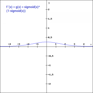
The gradient values are significant for range -3 and 3 but the graph gets much flatter in other regions. This implies that for values greater than 3 or less than -3, will have very small gradients. As the gradient value approaches zero, the network is not really learning.
Additionally, the sigmoid function is not symmetric around zero. So output of all the neurons will be of the same sign. This can be addressed by scaling the sigmoid function which is exactly what happens in the tanh function. Let’s read on.
4. Tanh
The tanh function is very similar to the sigmoid function. The only difference is that it is symmetric around the origin. The range of values in this case is from -1 to 1. Thus the inputs to the next layers will not always be of the same sign. The tanh function is defined as-
tanh(x)=2sigmoid(2x)-1
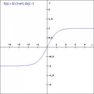
In order to code this is python, let us simplify the previous expression.
tanh(x) = 2sigmoid(2x)-1
tanh(x) = 2/(1+e^(-2x)) -1
And here is the python code for the same:
def tanh_function(x):
    z = (2/(1 + np.exp(-2*x))) -1
    return z
tanh_function(0.5), tanh_function(-1)
Output:
(0.4621171572600098, -0.7615941559557646)
As you can see, the range of values is between -1 to 1. Apart from that, all other properties of tanh function are the same as that of the sigmoid function. Similar to sigmoid, the tanh function is continuous and differentiable at all points.
Let’s have a look at the gradient of the tan h function.
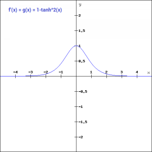
The gradient of the tanh function is steeper as compared to the sigmoid function. You might be wondering, how will we decide which activation function to choose? Usually tanh is preferred over the sigmoid function since it is zero centered and the gradients are not restricted to move in a certain direction.
5. ReLU
The ReLU function is another non-linear activation function that has gained popularity in the deep learning domain. ReLU stands for Rectified Linear Unit. The main advantage of using the ReLU function over other activation functions is that it does not activate all the neurons at the same time.
This means that the neurons will only be deactivated if the output of the linear transformation is less than 0. The plot below will help you understand this better-
f(x)=max(0,x)
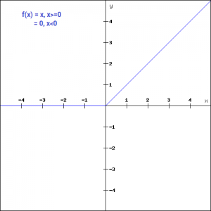
For the negative input values, the result is zero, that means the neuron does not get activated. Since only a certain number of neurons are activated, the ReLU function is far more computationally efficient when compared to the sigmoid and tanh function. Here is the python function for ReLU:
def relu_function(x):
    if x<0:
        return 0
    else:
        return x
relu_function(7), relu_function(-7)
Output:
(7, 0)
Let’s look at the gradient of the ReLU function.
f'(x) = 1, x>=0
      = 0, x<0
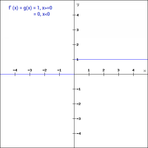
If you look at the negative side of the graph, you will notice that the gradient value is zero. Due to this reason, during the backpropogation process, the weights and biases for some neurons are not updated. This can create dead neurons which never get activated. This is taken care of by the ‘Leaky’ ReLU function.
6. Leaky ReLU
Leaky ReLU function is nothing but an improved version of the ReLU function. As we saw that for the ReLU function, the gradient is 0 for x<0, which would deactivate the neurons in that region.
Leaky ReLU is defined to address this problem. Instead of defining the Relu function as 0 for negative values of x, we define it as an extremely small linear component of x. Here is the mathematical expression-
f(x)= 0.01x, x<0
    =   x, x>=0
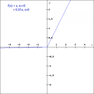
By making this small modification, the gradient of the left side of the graph comes out to be a non zero value. Hence we would no longer encounter dead neurons in that region. Here is the derivative of the Leaky ReLU function
f'(x) = 1, x>=0
     =0.01, x<0
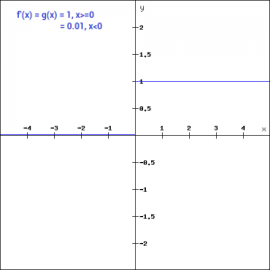
Since Leaky ReLU is a variant of ReLU, the python code can be implemented with a small modification-
def leaky_relu_function(x):
    if x<0:
        return 0.01*x
    else:
        return x
leaky_relu_function(7), leaky_relu_function(-7)
Output:
(7, -0.07)
Apart from Leaky ReLU, there are a few other variants of ReLU, the two most popular are – Parameterised ReLU function and Exponential ReLU.
7. Parameterised ReLU
This is another variant of ReLU that aims to solve the problem of gradient’s becoming zero for the left half of the axis. The parameterised ReLU, as the name suggests, introduces a new parameter as a slope of the negative part of the function. Here’s how the ReLU function is modified to incorporate the slope parameter-
f(x) = x, x>=0
    = ax, x<0
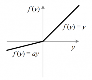
When the value of a is fixed to 0.01, the function acts as a Leaky ReLU function. However, in case of a parameterised ReLU function, ‘a‘ is also a trainable parameter. The network also learns the value of ‘a‘ for faster and more optimum convergence.
The derivative of the function would be same as the Leaky ReLu function, except the value 0.01 will be replcaed with the value of a.
f'(x) = 1, x>=0
      = a, x<0
The parameterized ReLU function is used when the leaky ReLU function still fails to solve the problem of dead neurons and the relevant information is not successfully passed to the next layer.
8. Exponential Linear Unit
Exponential Linear Unit or ELU for short is also a variant of Rectiufied Linear Unit (ReLU) that modifies the slope of the negative part of the function. Unlike the leaky relu and parametric ReLU functions, instead of a straight line, ELU uses a log curve for defning the negatice values. It is defined as
f(x) = x,   x>=0
    = a(e^x-1), x<0
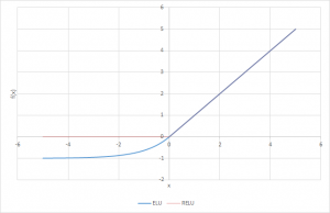
Let’s define this function in python
def elu_function(x, a):
    if x<0:
        return a*(np.exp(x)-1)
    else:
        return x
elu_function(5, 0.1),elu_function(-5, 0.1)
Output:
The derivative of the elu function for values of x greater than 0 is 1, like all the relu variants. But for values of x<0, the derivative would be a.e^x .
f'(x) = x,   x>=0
    = a(e^x), x<0
9.Swish
Swish is a lesser known activation function which was discovered by researchers at Google. Swish is as computationally efficient as ReLU and shows better performance than ReLU on deeper models. The values for swish ranges from negative infinity to infinity. The function is defined as –
f(x) = x*sigmoid(x)
f(x) = x/(1-e^-x)

As you can see, the curve of the function is smooth and the function is differentiable at all points. This is helpful during the model optimization process and is considered to be one of the reasons that swish outoerforms ReLU.
A unique fact about this function is that swich function is not monotonic. This means that the value of the function may decrease even when the input values are increasing. Let’s look at the python code for the swish function
def swish_function(x):
    return x/(1-np.exp(-x))
swish_function(-67), swish_function(4)
Output:
10. Softmax
Softmax function is often described as a combination of multiple sigmoids. We know that sigmoid returns values between 0 and 1, which can be treated as probabilities of a data point belonging to a particular class. Thus sigmoid is widely used for binary classification problems.
The softmax function can be used for multiclass classification problems. This function returns the probability for a datapoint belonging to each individual class. Here is the mathematical expression of the same-

While building a network for a multiclass problem, the output layer would have as many neurons as the number of classes in the target. For instance if you have three classes, there would be three neurons in the output layer. Suppose you got the output from the neurons as [1.2 , 0.9 , 0.75].
Applying the softmax function over these values, you will get the following result – [0.42 , 0.31, 0.27]. These represent the probability for the data point belonging to each class. Note that the sum of all the values is 1. Let us code this in python
def softmax_function(x):
    z = np.exp(x)
    z_ = z/z.sum()
    return z_
softmax_function([0.8, 1.2, 3.1])
Output:
array([0.08021815, 0.11967141, 0.80011044])
Choosing the right Activation Function
Now that we have seen so many activation functions, we need some logic / heuristics to know which activation function should be used in which situation. Good or bad – there is no rule of thumb.
However depending upon the properties of the problem we might be able to make a better choice for easy and quicker convergence of the network.
- Sigmoid functions and their combinations generally work better in the case of classifiers
- Sigmoids and tanh functions are sometimes avoided due to the vanishing gradient problem
- ReLU function is a general activation function and is used in most cases these days
- If we encounter a case of dead neurons in our networks the leaky ReLU function is the best choice
- Always keep in mind that ReLU function should only be used in the hidden layers
- As a rule of thumb, you can begin with using ReLU function and then move over to other activation functions in case ReLU doesn’t provide with optimum results
Projects
Now, its time to take the plunge and actually play with some other real datasets. So are you ready to take on the challenge? Accelerate your deep learning journey with the following Practice Problems:
Frequently Asked Questions
A. ReLU (Rectified Linear Activation) is a widely used activation function in neural networks. It introduces non-linearity, aiding in complex pattern recognition. By avoiding vanishing gradient issues, ReLU accelerates training convergence. However, its “dying ReLU” problem led to variations like Leaky ReLU, enhancing its effectiveness in deep learning models.
A. An activation function in neural networks determines the output of a neuron given its input. It introduces non-linearity, enabling the network to learn complex relationships. Common types include:
1. Sigmoid: S-shaped curve, suitable for binary classification but can suffer from vanishing gradient.
2. Tanh (Hyperbolic Tangent): Similar to sigmoid but centered around zero, still susceptible to vanishing gradient.
3. ReLU (Rectified Linear Activation): Replaces negative inputs with zero, addressing vanishing gradient and promoting faster training.
4. Leaky ReLU: Allows small negative values, avoiding the “dying ReLU” problem.
5. PReLU (Parametric ReLU): Generalizes Leaky ReLU by making the slope learnable.
6. ELU (Exponential Linear Unit): Smoothly handles negative inputs, preventing dead neurons and improving convergence.
7. Softmax: Converts a vector of scores into a probability distribution, often used in multi-class classification.
These functions enable neural networks to model complex data and make accurate predictions.
End Notes
In this article I have discussed the various types of activation functions and what are the types of problems one might encounter while using each of them.
I would suggest to begin with a ReLU function and explore other functions as you move further. You can also design your own activation functions giving a non-linearity component to your network. If you have used your own activation function which worked really well, please share it with us and we shall be happy to incorporate it into the list.


