Introduction
In this article, we will be taking a deep dive into an interesting algorithm known as “Seam Carving”. It does a seemingly impossible task of resizing an image without cropping it or distorting its contents. We will build our way up, to implement the seam carving algorithm from scratch while taking a peek at some of the interesting maths behind it.
Tad knowledge about calculus will be helpful to follow along but is not required. So let’s begin.
(This article is inspired by a lecture from Grant Sanderson at MIT.)
The Problem:
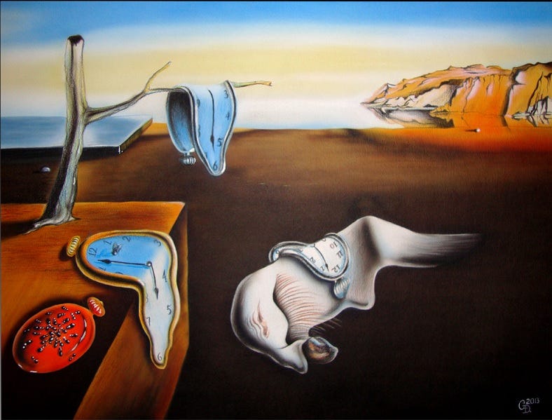
Let’s take a look at this image.
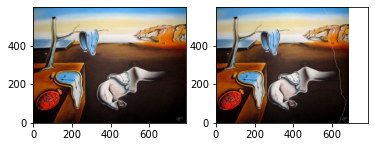
The painting, done by Salvador Dali, is named “The Persistence of Memory”. Rather than the artistic value, we are more interested in the contents of the painting. We want to resize the picture by decreasing its width. Two valid processes we can think of are cropping the picture or squeezing the width.
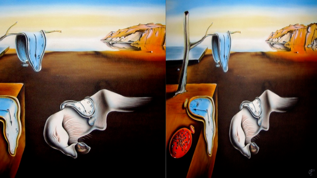
But as we can see, cropping removes many of the objects and squeezing distorts the pics. We want the best of both i.e. decrease the width without having to crop out any object or without distorting the objects.
As we can see, along with the objects, there are also a lot of empty spaces in the picture. What we want to accomplish here is to somehow remove those empty areas between the objects, so that the interesting parts of the picture remains while throwing away the unnecessary spaces.
This is indeed a tough problem, and it’s easy to get lost. So, it is always a good idea to split the problem into smaller more manageable parts. We can split this problem into two parts.
- Identifying interesting parts (i.e. objects) in the picture.
- Identifying pixel paths which can be removed without distorting the picture.
Identifying the Objects:
Before moving forward we would want to convert our picture to greyscale. It would be helpful for the operations we would be doing later. Here is a simple formula to convert an RGB pixel to a greyscale value.
def rgbToGrey(arr):
    greyVal = np.dot(arr[...,:3], [0.2989, 0.5870, 0.1140])
    return np.round(greyVal).astype(np.int32)
For identifying the objects, we can make a strategy. What if we can somehow identify all the edges in the picture? Then we can ask the seam carving algorithm to take the pixel paths which don’t travel through the edges so, by extension, any area closed by edges won’t be touched.
But then, how are we going to identify the edges? One observation we can make is, whenever there is a sharp change in color between two adjacent pixels, it’s most likely will be an edge to an object. We can rationalize this immediate change in color as the starting of a new object from that pixel.
The next problem we have to tackle is how to identify sharp changes in the pixel value. For now, let’s think of a simple case, a single line of pixels. Say we denote this array of values as x.
We may take the difference between the pixels x[i+1], x[i]. It would show how much our current pixel varies from the right-hand side. Or we can also take the difference of x[i] and x[i-1] which would give change on the left-hand side. For denoting the total change we may want to take the average of both, which yields,
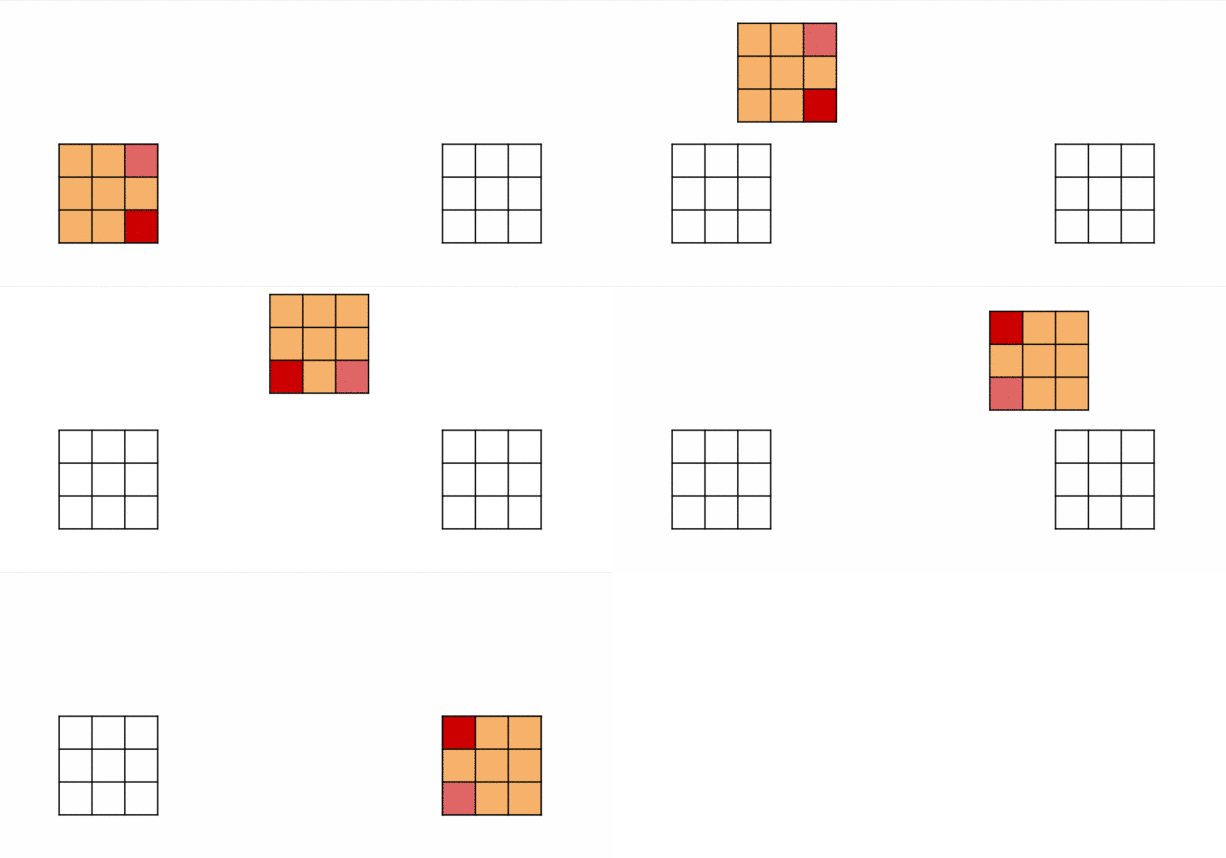
Anyone familiar with calculus can quickly identify this expression as the definition of a derivative. That’s right. We need to calculate the sharp change in x value so we are calculating the derivative of it. One more eager observation we can have is, if we define a filter say [-0.5,0,0.5] and took multiply it element-wise with the array [x[i-1],x[i],x[i+1]] and took its sum, it would give the derivative at x[i]. As our picture is 2d we would need a 2d filter. I won’t go into the details, but the 2d version of our filter looks like this,
As our filter calculates the derivative for each pixel along the x-axis it would give the vertical edges. Similarly, if we calculate the derivatives along the y-axis, we will have the horizontal edges. The filter for it would be the following. (It is the same as the filter for x-axis upon transpose.)
These filters are also known as Sobel Filters.
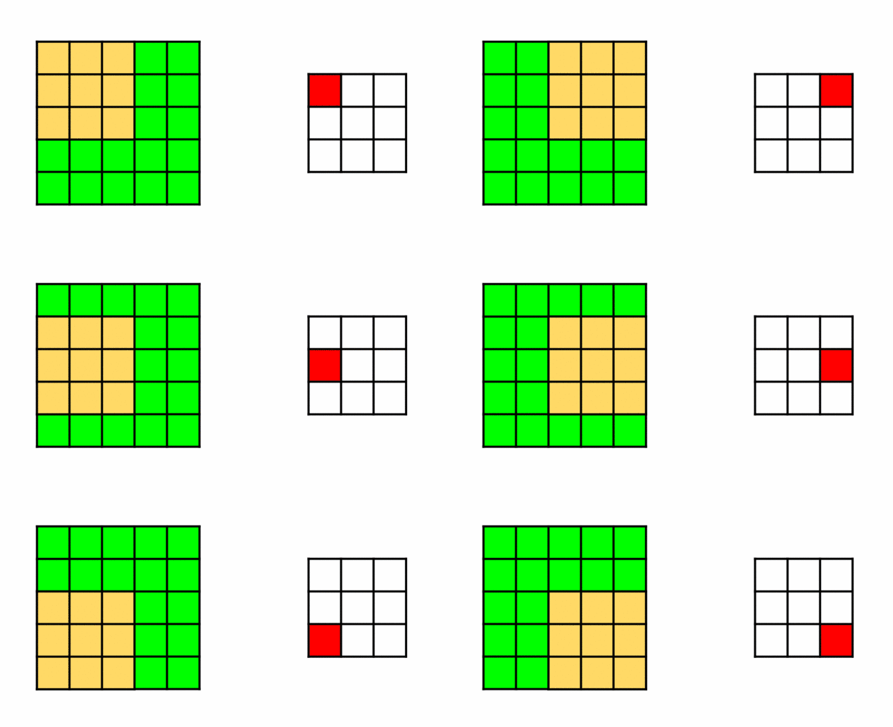
So, we have two filters that need to travel across the picture. For each pixel, doing an element-wise multiplication with (3X3) submatrix surrounding it then taking its sum. This operation is known as Convolution.
Convolution:
Mathematically the convolution operation is like this,
See how we do a pointwise multiplication of both functions then take its integration. Numerically it would correspond to what we did earlier i.e. element-wise multiplication of the filter and the image then taking the sum over it.
Notice, how for the k function it is written as k(t-τ). Because for the convolution operation one of the signals needs to be flipped. You can intuitively imagine it as something like this. Imagine two trains, on a straight horizontal track, are running towards each other for an inevitable collision (don’t worry nothing would happen to the trains because, Superposition). So the heads of the trains would be facing each other. Now imagine that you are scanning the track from left to right. Then for the left train, you would scan from rear to head.
Similarly, the computer needs to read our filters from the bottom-right (2,2) corner to the top-left (0,0) instead of from the top-left to the bottom-right. So the actual Sobel filters are the following,
upon which we do the 180-degree rotation before the convolution operation.
We can go on and write a simple naive implementation to do the convolution operation. It would be something like this,
def naiveConvolve(img,ker):

    res = np.zeros(img.shape)
    r,c = img.shape
    rK,cK = ker.shape
    halfHeight,halfWidth = rK//2,cK//2

    ker = np.rot90(ker,2)
    img = np.pad(img,((1,1),(1,1)),mode='constant')

    for i in range(1,r+1):
        for j in range(1,c+1):
            res[i-1,j-1] = np.sum(np.multiply(ker,img[i-halfHeight:i+halfHeight+1,j-halfWidth:j+halfWidth+1]))

    return res
This would work just fine but will take an excruciating amount of time to be executed, as it would be doing nearly 9*r*c multiplications and additions to arrive at the result. But we can be smart and use more concepts from math to decrease the time complexity drastically.
Fast Convolution:
Convolutions have an interesting property. Convolutions in the time domain correspond to multiplication over the frequency domain. I.e.
, where F(w) denotes the function in the frequency domain.
We know that Fourier transform converts a signal in the time domain to its frequency domain. So what we can do is, calculate the Fourier Transform of the image and the filter, multiply them, then take an Inverse Fourier Transform to get the convolution results. We can use the NumPy library for this.
def fastConvolve(img,ker):
    imgF = np.fft.rfft2(img)
    kerF = np.fft.rfft2(ker,img.shape)
    return np.fft.irfft2(imgF*kerF)
(Note: Values might be slightly different from the naive method in some cases, as the fastConvolve function calculates a circular convolution. But in practice we can comfortably use the fast convolution without worrying about these small differences in values.)
Cool! Now we have an efficient way to calculate the horizontal edges and the vertical edges, I.e the x and the y components. Thus, calculate the edges in the image using
def getEdge(greyImg):

    sX = np.array([[0.25,0.5,0.25],
                   [0,0,0],
                   [-0.25,-0.5,-0.25]])
    sY = np.array([[0.25,0,-0.25],
                   [0.5,0,-0.5],
                   [0.25,0,-0.25]])

    #edgeH = naiveConvolve(greyImg,sX)
    #edgeV = naiveConvolve(greyImg,sY)
    edgeH = fastConvolve(greyImg,sX)
    edgeV = fastConvolve(greyImg,sY)

    return np.sqrt(np.square(edgeH) + np.square(edgeV))
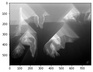
Awesome. We completed the first part. The edges are the interesting parts of the picture and the black parts are what we can remove without worrying.
Identifying Pixel Paths:
For a continuous path, we can define a rule that each pixel only connects to the 3 nearest pixels below it. This is to have a continuous path of pixels from top to bottom. So our subproblem becomes a basic pathfinding problem where we have to minimize the cost. As edges have higher magnitude, if we continue to remove the pixel paths with the lowest cost, it would avoid the edges.
Let’s define a function “cost” which takes a pixel and calculates the minimum cost pixel path to reach from there to the end of the pic. We have the following observations,
- In the bottom-most row (ie. i=r-1)
2. For any intermediate pixel,
Code:
def findCostArr(edgeImg):
    r,c = edgeImg.shape
    cost = np.zeros(edgeImg.shape)
    cost[r-1,:] = edgeImg[r-1,:]

    for i in range(r-2,-1,-1):

        for j in range(c):
            c1,c2 = max(j-1,0),min(c,j+2)
            cost[i][j] = edgeImg[i][j] + cost[i+1,c1:c2].min()

    return cost
Plot:
We can see the triangular shapes in the plot. They denote the points of no return, i.e. If you reach that pixel, there is no path to the bottom that doesn’t pass through an edge. And that is what we are trying to avoid.
From the cost matrix finding a pixel path can be easily done with a greedy algorithm. Find the min-cost pixel on the top row then move downwards selecting the pixel with the least cost among all the pixels connected to it.
def findSeam(cost):

    r,c = cost.shape

    path = []
    j = cost[0].argmin()
    path.append(j)

    for i in range(r-1):
        c1,c2 = max(j-1,0),min(c,j+2)
        j = max(j-1,0)+cost[i+1,c1:c2].argmin()
        path.append(j)

    return path
For removing the seam defined by the path we just have to go through each row and drop the column mentioned by the path array.
def removeSeam(img,path):
    r,c,_ = img.shape
    newImg = np.zeros((r,c,3))
    for i,j in enumerate(path):
        newImg[i,0:j,:] = img[i,0:j,:]
        newImg[i,j:c-1,:] = img[i,j+1:c,:]
    return newImg[:,:-1,:].astype(np.int32)
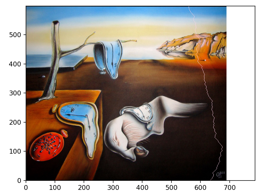
And, that is it. Here, I have pre-computed 100 seam carving operations.
We can see how the objects in the picture have come really close to each other. We have successfully decreased the size of the image using seam carving algorithm without causing any distortion to the objects. I have attached the link for the notebook with the full code. Interested readers can take a look here.
Overall, Seam Carving is a fun algorithm to play with. It does have it’s caveats as it will fail if the image provided has too many details or too many edges in it. It is always amusing to tinker around different pictures using the algorithm to see what the final result is. If you have any doubts or suggestions then kindly leave them in the responses. Thank you for reading until the end.


