Introduction
As data volume increases, deep learning techniques tend to perform better as compared to the classic methods. But, it comes with the drawback of complexity and thereby reduction in interpretability of the algorithm. The complexity also creates issues for hyperparameter tuning.
But what if there is a solution?
The solution is TENSORBOARD. It is a visualization extension created by the TensorFlow team to decrease the complexity of neural networks. Various types of graphs can be created using it. A few of those are Accuracy, Error, weight distributions, etc.
Components of Tensorboard
There are five components to it, namely:
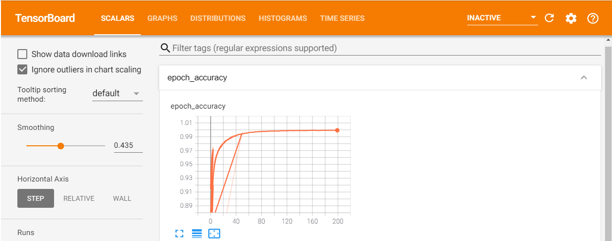
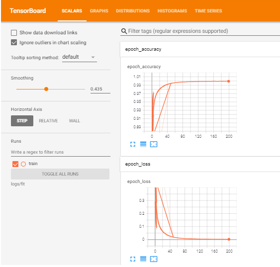
1) Scalars: It is very difficult to look at the accuracy and error for each epoch given the number of the epoch is very large and there are chances of ending up getting stuck in local minima instead of the global ones. These two problems can be solved using this section. It displays both accuracy and error graph wrt epoch.
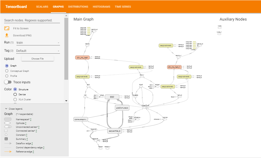
2) Graphs: This section visualizes the “model.summary()” results. In other words, it makes the architecture of neural networks more appealing. This eases the process of architecture understanding easier.
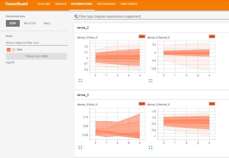
3) Distributions: In general, neural networks contain a lot of layers and every layer is composed of numerous biases and weights. This section represents the distribution of these hyperparameters.
4) Histograms: Consists of the histogram of these hyperparameters.
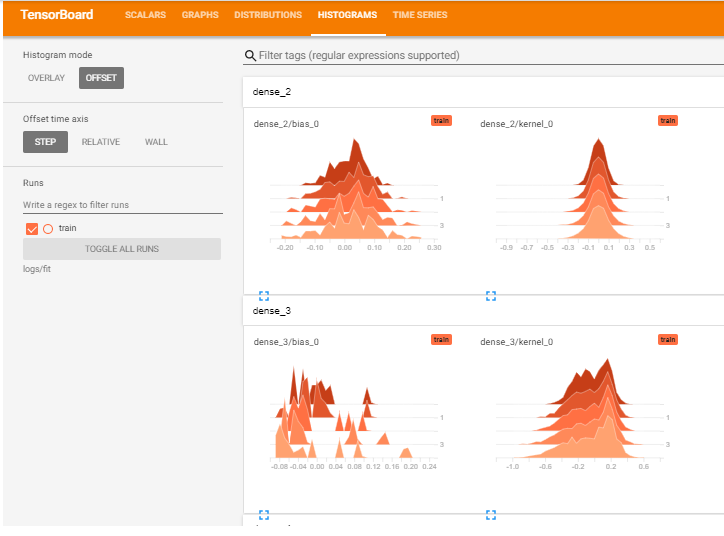
5) Time-Series: Consists of the over-time values for the same. These sections are useful in controlling the hyperparameters by analyzing their trends.
Code
There are two ways to publish tensorboards: localhost(powered by terminal) and within jupyter notebook. The below code looks at both scenarios. For this exercise, we will be taking a very famous inbuilt dataset: mnist.
Step 1: import the TensorFlow library.
import tensorflow as tf
Step 2: Load data and divide it into train and test
mnist = tf.keras.datasets.mnist
(x_train, y_train), (x_test, y_test) = mnist.load_data()
x_train, x_test = x_train / 255.0, x_test / 255.0
Step 3: Create model architecture
model = tf.keras.models.Sequential([
  tf.keras.layers.Flatten(input_shape=(28, 28)),
  tf.keras.layers.Dense(128, activation='relu'),
  tf.keras.layers.Dense(56, activation='relu'),
  tf.keras.layers.Dropout(0.2),
  tf.keras.layers.Dense(32, activation='relu'),
  tf.keras.layers.Dense(10)
])
Step 4: Compile model
model.compile(optimizer='SGD',
              loss=loss_fn,
              metrics=['accuracy'])
Step 5(important): Create a callback function. A callback function periodically(epochs) saves the model and the results(error, accuracy, bias, weights, etc) of the model. This is required as the graphs are a result of these values wrt every epoch.
tf_callbacks = tf.keras.callbacks.TensorBoard(log_dir = "logs/fit" , histogram_freq = 1)
Step 6(important): Model fitting (remember to pass callback function)
model.fit(x_train, y_train, epochs=200, callbacks = tf_callbacks)
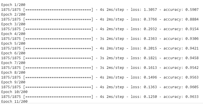
The results of these epochs are very difficult to remember.
Step 7: Create tensorboard using the following:
%reload_ext tensorboard
%tensorboard --logdir logs/fit
If this cod is entered into jupyter notebook, it will produce a board there. In case of hosting it over the localhost, put this in the command prompt(without “%”) and open this link: “https://localhost:6006”. Tensorboard gets launched on port number 6006.
Comparing optimizers using Tensorboard visualization
The performance of the two optimizers can also be compared through this. In order to do so, create two directories “logs/optimizer1″(step 5) and “logs/optimizer2” and use these directories to store the results of the respective optimizer(step 4 to change the optimizer and step 6 to execute that) and then launch the tensorboard using step 7.
Final Note:
Thanks for reading this blog, it requires a lot of patience to learn TensorFlow and its associated packages on your own. Kudos to you!
Please let me know of any questions/doubts you have regarding or anything related to machine learning. Share your feedback in the comments below.
You can reach out to me on LinkedIn as well 🙂
The media shown in this article are not owned by Analytics Vidhya and is used at the Author’s discretion.


