This article was published as a part of the Data Science Blogathon
Introduction
In this article, we will be learning how one of the deep learning technique used for finding the accuracy of the Breast Cancer Dataset, but I know that most of the techies are don’t know what we are talking about, We will start from the fundamental then we move ahead to our topic. First of all, we will take a brief introduction of deep learning then, what is Artificial Neural Network?
What is Deep learning?
If we talk about deep learning, then simply understand that it is a subset or subpart of machine learning. We can say that deep learning is an AI function that mimics the human brain and processes that data and creates patterns for use in decision making.
Deep learning is the type of machine learning which is something like the human brain, It uses a multi-layered structure of algorithms called neural networks. Its algorithms attempt to copy the data that humans would be analyzing the data with a given logical structure. It is also known as a deep neural network or deep neural learning.

In Deep learning there is one concept called Artificial Neural Network we will discuss briefly below:
Artificial Neural Network
As the name suggests artificial neural network, is the network of artificial neurons. It refers to a biologically inspired modeled after the brain. We can say that it is usually a computational network based on biological neural networks that construct the structure of the human brain.
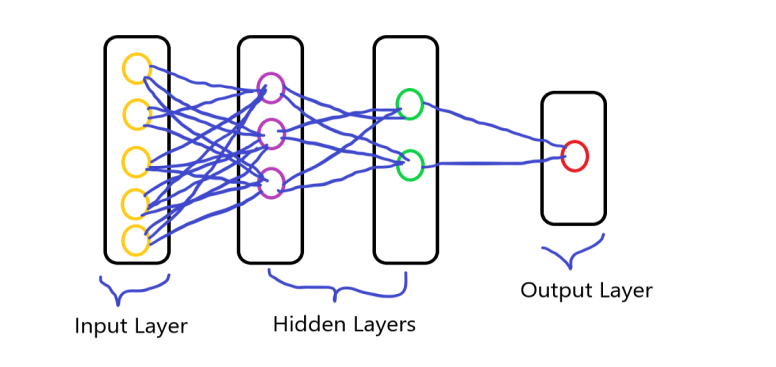
You all know that the neurons are interconnected with each other in our brains and the transmission of data process. It is similar to human brain neurons that are interconnected to each other, neural network consists of a large number of artificial neurons, which are termed units arranged in a sequence of layers. having the various layers of the neurons and forming a complete network. these neurons are termed nodes.
It is consist of three layers which is:
- Input layer
- Hidden layer
- Output layer
Create ANN Using Breast Cancer Dataset
Now we move to our topic, Here we will take the Dataset and then create the Artificial Neural Network and classify the diagnosis, for first, we take a dataset of breast cancer and then move forward.
Dataset: Breast Cancer Dataset
After downloading the dataset, we will import the important libraries that are required for the further process.
Import Libraries
#import pandas
import pandas as pd
#import numpy
import numpy as np
import matplotlib.pyplot as plt
import seaborn as sb
Here we import pandas, NumPy, and some visualization libraries.
Now we load our dataset using pandas:
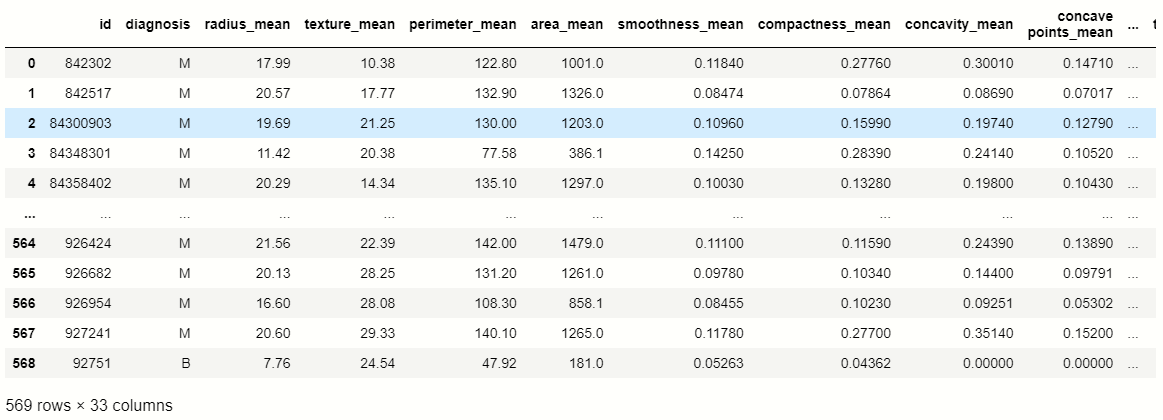
In this dataset, we point to the ‘diagnosis’ feature column, so we check the value count of that column using pandas:
# counting values of variables in 'diagnosis'
df['diagnosis'].value_counts()

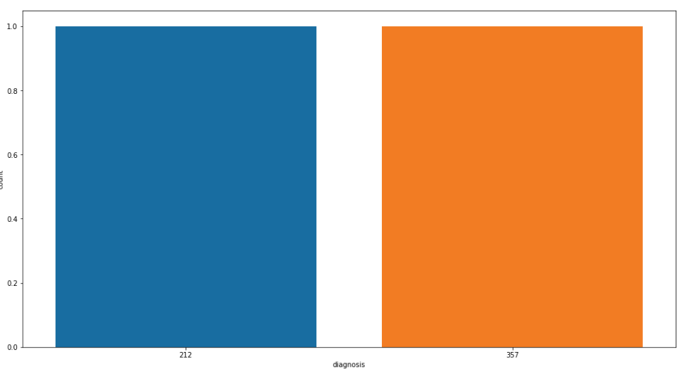
Now we visualize the value counts of the ‘diagnosis columns: for the better understanding
Visualize Value Counts
plt.figure(figsize=[17,9])
sb.countplot(df['diagnosis'].value_counts())
plt.show()
Null Values
In the dataset, we have to check that null values that are present inside the variables for that we use pandas:
df.isnull().sum()
After executing the program we reach the conclusion that the feature name ‘Unnamed:32’ contains all the null values so we delete or drop that column.
#droping feature
df.drop(['Unnamed: 32','id'],axis=1,inplace=True)
Independent and Dependent Variables
Now it’s time for dividing the dataset into independent and dependent variables, for that we create two variables one represents independent and the other represents dependent.
# independent variables
x = df.drop('diagnosis',axis=1)
#dependent variables
y = df.diagnosis
Handling Categorical Value
When we print the dependent variable y then we see that there contain categorical data and we have to convert categorical data into the binary format for further process, So we use Scikit learn Label Encoder for encoding the categorical data.
from sklearn.preprocessing import LabelEncoder
#creating the object
lb = LabelEncoder()
y = lb.fit_transform(y)
Splitting Data
Now its time for splitting the data into training and testing parts:
from sklearn.model_selection import train_test_split
xtrain,xtest,ytrain,ytest = train_test_split(x,y,test_size=0.3,random_state=40)
Scaling the Data
When we create the artificial neural network, then we have to scale the data into smaller numbers because the deep learning algorithm multiplies the weights and input data of the nodes and it takes lots of time, So for reducing that time we scale the data.
For scaling, we use the scikit learn StandardScaler module, we scale the training and testing dataset:
#importing StandardScaler
from sklearn.preprocessing import StandardScaler
#creating object
sc = StandardScaler()
xtrain = sc.fit_transform(xtrain)
xtest = sc.transform(xtest)
From here we start creating the artificial neural network, for that we import the important libraries that are used for creating ANN:
#importing keras
import keras
#importing sequential module
from keras.models import Sequential
# import dense module for hidden layers
from keras.layers import Dense
#importing activation functions
from keras.layers import LeakyReLU,PReLU,ELU
from keras.layers import Dropout
Creating Layers
After importing those libraries, we create the three types of layers:
- Input layer
- Hidden layer
- Output layer
First, we create the model:
#creating model
classifier = Sequential()
A sequential model is appropriate for a plain stack of layers where each layer has exactly one input tensor and one output tensor.
Now we create the layers of the neural network:
#first hidden layer
classifier.add(Dense(units=9,kernel_initializer='he_uniform',activation='relu',input_dim=30))
#second hidden layer
classifier.add(Dense(units=9,kernel_initializer='he_uniform',activation='relu'))
# last layer or output layer
classifier.add(Dense(units=1,kernel_initializer='glorot_uniform',activation='sigmoid'))
In the following code, the Dense method is used for creating the layers, in that we use fundamental parameters. The first parameter is Output Nodes, the Second is the initializer for the kernel weights matrix, the Third is Activation function and the last parameter is input nodes or the number of independent features.
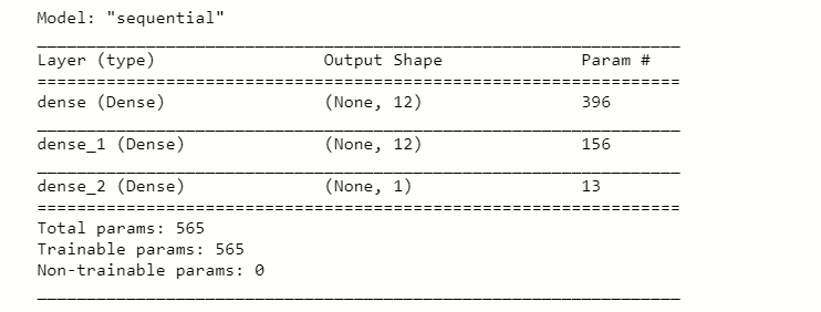
After executing this code we take the summary of it using :
#taking summary of layers
classifier.summary()
Compiling ANN
Now we compiling our model with the optimizer:
#compiling the ANN
classifier.compile(optimizer='adam',loss='binary_crossentropy',metrics=['accuracy'])
Fitting the ANN Into Training Data
After compiling the model we have to fit the ANN into the training data for the prediction:
 #fitting the ANN to the training set
model = classifier.fit(xtrain,ytrain,batch_size=100,epochs=100)
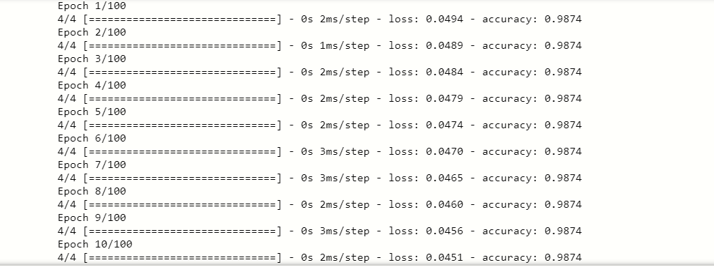
The fit() method fits the ANN to the training data, in the parameters we set the specific values of each variable like batch_size, epochs, etc… At last, we find an excellent accuracy score, So our model fir perfectly into training data.
After training data we have to test the accuracy score for the Test data also, let’s see below:
#now testing for Test data
y_pred = classifier.predict(test)
On executing this code we find that y_pred contained the different values so we converting the predicting values into the threshold values like True, False.
#converting values
y_pred = (y_pred>0.5)
print(y_pred)

Score and Confusion Matrix
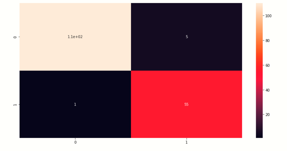
Now we check the confusion matrix and the score of the predicted values.
from sklearn.metrics import confusion_matrix
from sklearn.metrics import accuracy_score
cm = confusion_matrix(ytest,y_pred)
score = accuracy_score(ytest,y_pred)
print(cm)
print('score is:',score)
Output:-

Visualize Confusion Matrix
Here we visualize the confusion matrix of the predicting values
# creating heatmap of comfussion matrix
plt.figure(figsize=[14,7])
sb.heatmap(cm,annot=True)
plt.show()
Visualize Data History
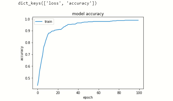
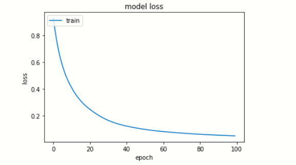
Now we visualize the loss and accuracy in each epoch.
# list all data in history
print(model.history.keys())
# summarize history for accuracy
plt.plot(model.history['accuracy'])
plt.title('model accuracy')
plt.ylabel('accuracy')
plt.xlabel('epoch')
plt.legend(['train', 'test'], loc='upper left')
plt.show()
# summarize history for loss
plt.plot(model.history['loss'])
plt.title('model loss')
plt.ylabel('loss')
plt.xlabel('epoch')
plt.legend(['train', 'test'], loc='upper left')
plt.show()
Saving Model
At last, we save our model
#saving the model
classifier.save('File_name.h5')
EndNote
This is my first ANN created in deep learning, I am a beginner in deep learning I try my best to explain this article hope you like this article. Thank you for reading this article.😊
Connect with me on LinkedIn: Profile
Thank You.
The media shown in this article are not owned by Analytics Vidhya and are used at the Author’s discretion.


