This article was published as a part of the Data Science Blogathon
Introduction
Unsupervised learning, where there are no predefined labels for the data and the model segments the data into groups by inferring patterns and extracting features from the data, is at the heart of the data science problems. In the machine learning world, Segmentation helps to cluster the data based on their characteristics.
Similar to Segmentation, a parallel technique exists in the realm of deep learning which is called Self Organizing Maps. In this article, we will dive deep into this technique in detail, covering what is Self Organizing Maps, their architecture, how they are trained, what their applications are, how is it similar to K-Means Clustering, and then implement in Python.
Table of Contents
- What are Self-Organizing Maps?
- The architecture of Self-Organizing Maps
- How do Self-Organizing Maps learn?
- Best Matching Unit (BMU)
- The Analogy of Self-Organizing Maps to K-means Clustering
- Implementation of Self-Organizing Maps on Python
What are Self-Organizing Maps?
Invented by Prof. Teuvo Kohonen, Kohonen artificial neural networks or Kohonen maps is another breed of Artificial Neural Networks (ANNs). More famously known as the Self-Organizing Map (SOMs) it is a very rare facet of unsupervised learning and is a data visualization technique.
The goal of the technique is to reduce dimensions and detect features. The maps help to visualize high-dimensional data. It represents the multidimensional data in a two- dimensional space using the self-organizing neural networks. The technique is used for data mining, face recognition, pattern recognition, speech analysis, industrial and medical diagnostics, anomalies detection.
The beauty of SOMs is that it preserves the topological relationship of the training dataset (or the input). Implying that the underlying properties of the input data are not affected even after the continuous change in the shape or the size of the figure. SOMs help to reveal correlations that are not easily identified.
Lets’ see how the SOMs are structured and understanding their architectural nuances …
The Architecture of Self-Organizing Maps
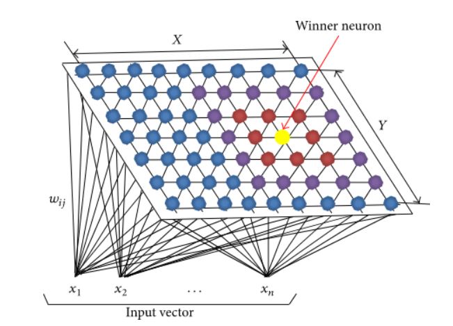
The self-organizing maps structure is a lattice of neurons. In the grid, X and Y coordinate, each node has a specific topological position and comprises a vector of weights of the same dimension as that of the input variables.
The input training data is a set of vectors of n dimensions: x1, x2, x3…xn, and each node consists of a corresponding weight vector W of n dimensions: w1, w2, w3… wn
In the illustration below, the lines between the nodes are simply a representation of adjacency and not signifying any connection as in other neural networks.

Image 1
Self-Organizing Maps are a lattice or grid of neurons (or nodes) that accepts and responds to a set of input signals. Each neuron has a location, and those that lie close to each other represent clusters with similar properties. Therefore, each neuron represents a cluster learned from the training.
In SOMs, the responses are compared and a ‘winning’ neuron is selected from the lattice. This selected neuron is activated together with the neighbourhood neurons. SOMs return a two-dimensional map for any number of indicators as output where there are no lateral connections between output nodes.
Here’s a question for you, what do you think is the loss function that needs to be computed for SOMs? Well, as it is an unsupervised learning technique, there is no target variable and hence, we do not even calculate the loss function and therefore there is no backward propagation process also needed for SOMs.
How do Self-Organizing Maps Learn?
Now, let’s understand what is the learning mechanism of the self-organizing maps algorithm? How are the betas estimated and the network gets trained?
The underlying idea of the SOMs training process is to examine every node and find the one node whose weight is most like the input vector. The training is carried out in a few steps and over many iterations. Let’s see this in detail below:
We have three input signals x1, x2, and x3. This input vector is chosen at random from a set of training data and presented to the lattice. So, we have a lattice of neurons in the form of a 3*3 two-dimensional array having nine nodes with three rows and three columns depicted like below:
Image 2
For understanding purposes, visualize the above 3*3 matrix as below:
Image 3
Each node has some random values as weights. These weights are not of the neural network as shown as:
Image 4
From these weights, can calculate the Euclidean distance as:
Image 5
The training process of SOMs follows:
-
Firstly, randomly initialize all the weights.
-
Select an input vector x = [x1, x2, x3, … , xn] from the training set.
-
Compare x with the weights wj by calculating Euclidean distance for each neuron j. The neuron having the least distance is declared as the winner. The winning neuron is known as Best Matching Unit(BMU)
-
Update the neuron weights so that the winner becomes and resembles the input vector x.
-
The weights of the neighbouring neuron are adjusted to make them more like the input vector. The closer a node is to the BMU, the more its weights get altered. The parameters adjusted are learning rate and neighbourhood function. (more below on neighbourhood function)
-
Repeat from step 2 until the map has converged for the given iterations or there are no changes observed in the weights.
Best Matching Unit (BMU)
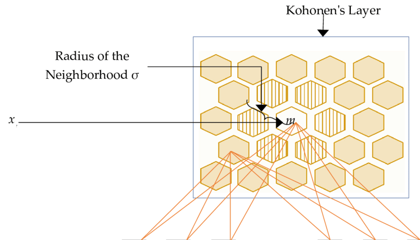
As we saw above the distance of each of the nodes (or raw data point) is calculated from all the output nodes. The node or neuron which is identified with the least distance is the Best Matching Unit (BMU) or neighbourhood. It is depicted as (m) in the following figure:

Image 6
From this BMU, a radius (or sigma) is defined. All the nodes that fall in the radius of the BMU get updated according to their respective distance from the BMU.
So, now the point is that a neuron in the output map can be a part of the radius of many different Best Matching Units. This leads to a constant push and pulls effect on the neuron however, the behaviour of the neuron will be more similar to the Best Matching Unit near it.
After each iteration, the radius shrinks and the BMU pulls lesser nodes so the process becomes more and more accurate and that shrinks the neighbourhood that reduces the mapping of those segments of those data points which belong to that particular segment. This makes the map more and more specific and ultimately it starts converging and becomes like the training data (or input).

Image 7
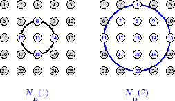
In the above figure, the radius of the neighbourhood of the Best Matching Unit (BMU) is calculated. This is a value that starts large as on the right side of the panel, typically set to the radius of the lattice but diminishes each time step. Any nodes found within this radius are deemed to be inside the BMU’s neighbourhood.
The Analogy of SOMs to K-means Clustering
Both K-Means clustering and SOMs are a means to convert the higher dimensional data to lower dimensional data. Though one is a machine learning algorithm and another is a deep learning algorithm yet there is an analogy between the two.
In K-Means clustering, when new data points are presented, the centroids are updated and there are methods such as the elbow method to find the value of K. Whereas in Self Organizing Maps, the architecture of the neural network is changed to update the weights and the number of neurons is a tuning parameter.
Implementation of Self-Organizing Maps on Python
We shall employ the self-organizing maps technique to detect fraud customers in Python. The data has 690 records and 16 features along with a class label and customerID. Since SOMs are an unsupervised technique, we wouldn’t be using the class column here and also do not need the customerID column. The dataset and codes can be accessed from my GitHub repository.
The SOMs return a two-dimensional map where colour-coding is employed to map the identified specific group of data points.
In Python, we use the library called Minisom is used for performing Self Organizing Maps.
import numpy as np

import matplotlib.pyplot as plt

import pandas as pd

# Minisom library and module is used for performing Self Organizing Maps

from minisom import MiniSom
# Loading Data

data = pd.read_csv('Credit_Card_Applications.csv')

# X

data

# Shape of the data:

data.shape

# Info of the data:

data.info()
For Self Organizing Maps, only require X variables. In this case, we do not require the customerID as it is a unique variable and neither the Y (target variable) hence not using either.
Though, the target variable (Y) can be used to understand if the output is matching with input or not.
# Defining X variables for the input of SOM
X = data.iloc[:, 1:14].values
y = data.iloc[:, -1].values
# X variables:
pd.DataFrame(X)
Scaling the X variables:
from sklearn.preprocessing import MinMaxScaler
sc = MinMaxScaler(feature_range = (0, 1))
X = sc.fit_transform(X)
pd.DataFrame(X)
SOMs are a two-dimensional array of neurons. So, to define the SOMs we would require to know how many rows and columns and neurons are needed in order of the x and y dimensions. The parameters of SOM are:
- x: som_grid_rows, is the number of rows
- y: som_grid_columns, is the number of columns
- Sigma is the neighborhood radius
- learning_rate
As x and y are the dimensions of the SOM, these should not be small and Sigma and learning_rate can be taken higher values because in every iteration these values are adjusted. Though the initial value of the radius is 1.
# Set the hyper parameters
som_grid_rows = 10
som_grid_columns = 10
iterations = 20000
sigma = 1
learning_rate = 0.5
With x = 10 and y = 10 as the respective number of rows and number of columns (dimensions), there will be 10* 10 meaning 100 segments. We randomly take the observations and not in any sequence to perform the iterations.
# define SOM:

som = MiniSom(x = som_grid_rows, y = som_grid_columns, input_len=13, sigma=sigma, learning_rate=learning_rate)

# Initializing the weights

som.random_weights_init(X)

# Training

som.train_random(X, iterations)
The weights and distance map from the weights are:
# Weights are:
wts = som.weights
# Shape of the weight are:
wts.shape
# Returns the distance map from the weights:
som.distance_map()
We compute the Mean Inter-Neuron Distance(MID), which is the mean Euclidean distance of the main neuron with its neighbourhood.
- The higher the MID, the more away will be the winning node from its neighbourhood.
- The Best Matching Unit far from its neighbourhood is generally far from the clusters.
- If some values have more similar distances i.e small distances in terms of the MID then those values are more closer and similar to each other.
Pcolor() is used to colour all MIDs and the window is the bone().
from pylab import plot, axis, show, pcolor, colorbar, bone
bone()
pcolor(som.distance_map().T)       # Distance map as background
colorbar()
show()
Using different colors and markers for each label for identifying the patients with the disease. The most common example used to explain SOM principles is the mapping of colors from the three dimension-red, green-blue into two dimensions. If the outlier depicted in the heatmap is aligned or not with the actual fraud customers then can cross-check via:
bone()

pcolor(som.distance_map().T)

colorbar() #gives legend

markers = ['o', 's']                     # if the observation is fraud then red circular color or else green square

colors = ['r', 'g']

for i, x in enumerate(X):

    w = som.winner(x)

    plot(w[0] + 0.5,

         w[1] + 0.5,

         markers[y[i]],

         markeredgecolor = colors[y[i]],

         markerfacecolor = 'None',

         markersize = 10,

         markeredgewidth = 2)

show()
- The markers used to distinguish frauds are:
- Red Circular is Class 0 as fraud customers
- Green Square is Class 1 as not fraud customers
- i is the index and x is the vector of each value and for each x first get the winning node
- The co-ordinates of the winning node are w[0] and w[1], 0.5 is added to center the marker
- s is a square and marker face color is the inside color of the marker
There will be some customers who do not have any mapping above and hence those would not be part of the segments. For showing the values forming part of the segments:
mappings = som.win_map(data)

mappings

mappings.keys()

len(mappings.keys())

mappings[(9,8)]

Taking some of the red circulars from the heat map and mapping as frauds:
frauds = np.concatenate((mappings[(0,9)], mappings[(8,9)]), axis = 0)

frauds

# the list of customers who are frauds:

frauds1 = sc.inverse_transform(frauds)

pd.DataFrame(frauds1)
Endnotes
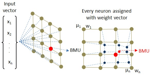
The below schematic illustrates the working of the self-organizing maps:

Image 8
-
The self-organizing maps algorithm projects the high-dimensional data into a two- dimensional map while retaining the topology of the data so that similar data points are mapped to the nearby locations on the map.
-
The technique classifies the data without any supervision and there is no target vector and hence no backward propagation.
-
The output of the SOMs is a two-dimensional map and color-coding is used to identify any specific group of data points.
I hope the article was helpful to you and you learned something new. Thank You so much for stopping by to read and helping in sharing the article with your network 🙂
Happy Learning! 🙂
About me
Hi there! I am Neha Seth. I hold a Postgraduate Program in Data Science & Engineering from the Great Lakes Institute of Management and a Bachelors in Statistics. I have been featured as Top 10 Most Popular Guest Authors in 2020 on Analytics Vidhya (AV).
My area of interest lies in NLP and Deep Learning. I have also passed the CFA Program. You can reach out to me on LinkedIn and can read my other blogs for AV.
References
https://en.wikipedia.org/wiki/Teuvo_Kohonen
Image Sources
- Image 1: https://static-01.hindawi.com/articles/cin/volume-2016/2476256/figures/2476256.fig.002.svgz
- Image 2: 63_blog_image_2.png (671×663) (sds-platform-private.s3-us-east-2.amazonaws.com)
- Image 3 : 63_blog_image_3.png (671×663) (sds-platform-private.s3-us-east-2.amazonaws.com)
- Image 4 : 63_blog_image_4.png (671×663) (sds-platform-private.s3-us-east-2.amazonaws.com)
- Image 5 : 63_blog_image_5.png (671×663) (sds-platform-private.s3-us-east-2.amazonaws.com)
- Image 6: https://www.researchgate.net/publication/350552111/figure/fig2/AS:1007773596786688@1617283357172/The-best-matching-unit-in-the-Self-Organizing-Map-SOM.png
- Image 7: mathworks.com
- Image 8: https://www.researchgate.net/profile/Bruno-Senzio/publication/313160273/figure/fig2/AS:456827105222657@1485927477162/SOM-Structure-and-Update-of-Best-Matching-Unit-19.png
The media shown in this article are not owned by Analytics Vidhya and are used at the Author’s discretion.


