This article was published as a part of the Data Science Blogathon
Why Neural Networks? How do Neural Networks do what they do? How does Forward Propagation work?
Neural Networks can be thought of as a function that can map between inputs and outputs. In theory, no matter how complex that function is, neural networks should be able to approximate that function. However, most supervised learning, if not all, is about learning a function that maps given X and Y And later using that function to find the appropriate Y for a new X. If so, what is the difference between traditional machine learning algorithms and neural networks? The answer is something known as Inductive Bias. The term might look new. But, it is nothing but the assumptions that we place upon the relationship between X and Y before fitting a machine learning model into it.
For example, if we think the relationship between X and Y is linear, we could use linear regression. The Inductive Bias of linear regression is that the relationship between X and Y is linear. Hence, it fits a line or a hyperplane to the data.
But when a non-linear and complex relationship exists between the X and Y, a linear regression algorithm might not do a great job in predicting Y. In this case, we might require a curve or a multi-dimensional curve to approximate that relationship. The main advantage of neural networks is it’s Inductive Bias is very weak and hence, no matter how complex this relationship or function is, the network is somehow able to approximate it.
But also, based on the complexity of the function, we might have to manually set the number of neurons in each layer and the number of layers in the network. This is usually done by trial and error and experience. hence, these parameters are called hyperparameters.
Neural networks are nothing but complex curve-fitting machines. — Josh Starmer
Architecture and working of neural networks
before we see why whatever neural networks works, it would be appropriate to show what neural networks do. before understanding the architecture of a neural network, we need to look into what a neuron does first.
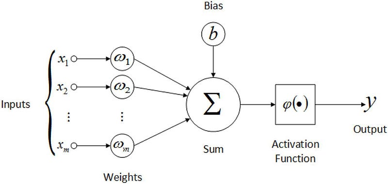
Each Input to an artificial neuron has a weight associated with it. The inputs are first multiplied with their respective weights and a bias is added to the result. we can call this the weighted sum. The weighted sum then goes through an activation function, which is basically a non-linear function.
So, An artificial neuron can be thought of as a simple or multiple linear regression model with an activation function at the end. Having said that, let’s move on to neural network architecture
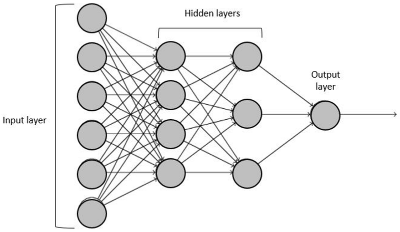
A neural network typically has multiple layers with each layer having multiple neurons, where all the neurons from one layer are connected to all the neurons in the next layer and so on.
In fig 1.2, we have 4 layers. The first layer is the input layer which looks like it contains 6 neurons, but in reality, it is nothing but the data that is served as input to the neural network ( There are 6 neurons because the input data probably has 6 columns). The final layer is the output layer. The number of neurons in the final layer and the first layer is predetermined by the dataset and the type of problem (number of output classes and such). The number of neurons in the hidden layers and the number of hidden layers are to be chosen by trial and error.
A neuron from layer i will take the output of all the neurons from layer i-1 as inputs and calculates the weighted sum adds a bias to it, and then finally, send it through an activation function, as we saw above in the case of an artificial neuron. The first neuron from the first hidden layer will be connected to all the inputs from the previous layer ( input layer). similarly, the second neuron from the first hidden layer will also be connected to all the inputs from the previous layer, and so on for all the neurons in the first hidden layer. For neurons in the second hidden layer, outputs of the previously hidden layer are considered as the inputs and each of these neurons is connected to all the previous neurons, likewise.
a layer with m neurons, preceded by a layer with n neurons would have n*m + m (including bias) connections or links with each link carrying a weight. These weights are initialized randomly but on training, they reach their optimal value so as to reduce the loss function we choose. we will see about learning these weights in detail in the upcoming blog.
Example of Forward Propagation
Let us consider the neural network we have in fig 1.2 and then show how forward propagation works with this network for better understanding. We can see that there are 6 neurons in the input layer which means there are 6 inputs.
Note: For calculation purposes, I am not including the biases. But, if biases were to be included, There simply will be an extra input I0 whose value will always be 1 and there will be an extra row at the beginning of the weight matrix w01, w02….w04
Let the inputs be I = [ I1, I2, I3, I4, I5, I6 ]. we can see that the first hidden layer has 4 neurons. So, there are going to be 6*4 connections (without bias) between the input layer and the first hidden layer. These connections have been represented in green color in the below weight matrix with values w_ij which represents the weight for the connection between ith neuron from the input layer and jth neuron from the first hidden layer. If we multiply (matrix multiplication) the 1*6 input matrix with the 6*4 weight matrix, we will get the outputs from the first hidden layer which is 1*4. This makes sense because there are literally 4 neurons in the first hidden layer.
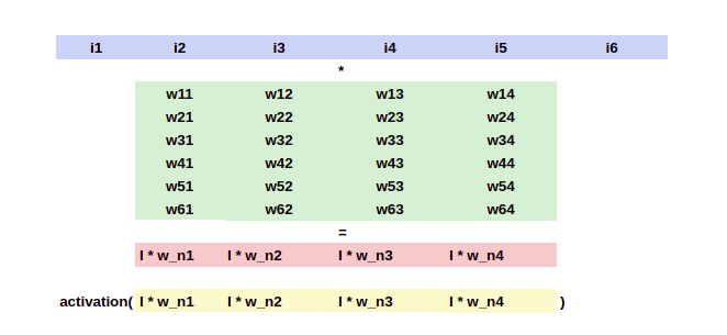
These 4 outputs are represented in the color red in fig 2.1. Once these values are obtained, we send them through an activation function in order to introduce non-linearity and then, those values will be the exact output of the first hidden layer.
Now, we continue the same steps for the second hidden layer with a different weight matrix for it.
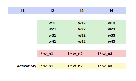
The i1, i2,etc. are nothing but the outputs of the previous layer. I am using the same variable I for ease of understanding. Similar to what we have previously seen, the input 1*4 matrix is going to be multiplied with the 4*3 weight matrix (because the second hidden layer has 3 neurons), which output a 1*3 matrix. The activation of the individual elements in that matrix will be the input for the next layer.
Take a small guess at the shape of the weight matrix for the final layer

As the final layer has only 1 neuron and the previous layer has 3 outputs, the weight matrix is going to be of size 3*1, and that marks the end of forwarding propagation in a simple feed-forward neural network.
Why this approach works?
We already saw what each neuron in the network does is not so different from a linear regression. In addition, the neuron adds an activation function at the end and each neuron has a different weight vector. But, why does this work?
Now we have already seen how the calculation works. But, my main goal with this blog is to shed some light on why this approach works. In theory, neural networks should be able to approximate any continuous function, however complex and non-linear it is. I am going to try my best to convince you, and myself that, with the right parameters (weights and biases), the network should be able to learn anything with the approach we saw above.
Importance of Non-Linearity
Before we go further, we need to understand the power of non-linearity. When we add 2 or more linear objects like a line, plane, or hyperplane, the resultant is also a linear object: line, plane, or hyperplane respectively. No, matter in what proportion we add these linear objects, we are still going to get a linear object.
But, this is not the case for addition between non-linear objects. when we add 2 different curves, we are probably going to get a more complex curve. This is shown in the below gist. If we could add different parts of these non-linear curves with different proportions, we should somehow be able to influence the shape of the resultant curve.
In addition to just adding non-linear objects or let’s say “hyper-curves” like “hyperplanes”, we are also introducing non-linearity at every layer through these activation functions. which basically means, we are applying a non-linear function over an already non-linear object. And by tuning these biases and weights, we are able to change the shape of the resultant curve or function.
This is the reason that more complex problems require more hidden layers and more hidden neurons and less complex problems or relationships can be approximated with a lesser number of layers and neurons. Each neuron acts as a problem-solver. They all solve their own small problems and in combination, they solve a bigger problem which is usually to reduce the cost function. The exact word to use here is Divide and Conquer.
What if Neural networks didn’t use Activation functions?
If neural networks didn’t use an activation function, it’s just going to be a big linear unit, which could be easily replaced by a single linear regression model.
y = m*x + c
z = k*y + t => k*(m*x+c) + t => k*m*x + k*c + t => (k*m)*x + (k*c+t)
Here, Z is also linearly dependent on x as k*m can be replaced with another variable, and k*c+t can be replaced with one more variable. hence, without activation functions, no matter how many layers and how many neurons there are, all of those are going to be redundant.
Conclusion
We saw how neural networks calculate their outputs and why that method works. To put it simply, the main reason behind why neural networks are able to learn complex relationships is because at each and every layer we introduce non-linearity and add different proportions of the output curve in order to get the desired result and this result also goes through an activation function and the same process is repeated to further customize the resultant. all the weights and biases in the network are important and they can be adjusted in certain ways to approximate the relationship. even though the weights assigned to each neuron are random initially, they will be learned through a special algorithm called backpropagation.
FAQs
CNNs are specifically designed for image recognition tasks, while FFNNs are more general-purpose ANNs. CNNs use convolutional layers to extract features from images, while FFNNs use fully connected layers to process information.
Feed-forward networks are simple and versatile artificial neural networks that can be used for a variety of tasks, including classification, regression, and function approximation. They are easy to train and understand, but they may not be able to capture sequential dependencies or handle complex tasks.
FFNNs are simple, versatile, efficient, robust, adaptable, interpretable, and widely available, making them a valuable tool for machine learning.


