Originally posted by Manojit Nandi, Data Scientist at STEALTHbits Technologies on the Domino data science blog
Domino recently added support for GPU instances. To celebrate this release, I will show you how to:
Configure the Python library Theano to use the GPU for computation.
Build and train neural networks in Python.
Using the GPU, I’ll show that we can train deep belief networks up to 15x faster than using just the CPU, cutting training time down from hours to minutes. You can see my code, experiments, and results on Domino.
Why are GPUs useful?
When you think of high-performance graphics cards, data science may not be the first thing that comes to mind. However, computer graphics and data science have one important thing in common: matrices!
Images, videos, and other graphics are represented as matrices, and when you perform a certain operation, such as a camera rotation or a zoom in effect, all you are doing is applying some mathematical transformation to a matrix.
What this means is that GPUs, compared to CPUs (Central Processing Unit), are more specialized at performing matrix operations and other advanced mathematical transformations. In some cases, we see a 10x speedup in an algorithm when it runs on the GPU.
GPU-based computation have been employed in a wide variety of scientific applications, from genomic to epidemiology
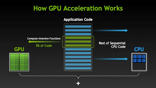
Recently, there has been a rise in GPU-accelerated algorithms in machine learning thanks to the rising popularity of deep learning algorithms. Deep Learning is a collection of algorithms for training neural network-based models for various problems in machine learning. Deep Learning algorithms involve computationally intensive methods, such as convolutions, Fourier Transforms, and other matrix-based operations which GPUs are well-suited for computing. The computationally intensive functions, which make up about 5% of the code, are run on the GPU, and the remaining code is run on the CPU.
With the recent advances in GPU performance and support for GPUs in common libraries, I recommend anyone interested in deep learning get ahold of a GPU.
Now that I have thoroughly motivated the use of GPUs, let’s see how they can be used to train neural networks in Python.
Deep Learning in Python
The most popular library in Python to implement neural networks is Theano. However, Theano is not strictly a neural network library, but rather a Python library that makes it possible to implement a wide variety of mathematical abstractions. Because of this, Theano has a high learning curve, so I will be using two neural network libraries built on top of Theano that have a more gentle learning curve.
The first library is Lasagne. This library provides a nice abstraction that allows you to construct each layer of the neural network, and then stack the layers on top of each other to construct the full model. While this is nicer than Theano, constructing each layer and then appending them on top of one another becomes tedious, so we’ll be using the Nolearn library which provides a Scikit-Learn style API over Lasagne to easily construct neural networks with multiple layers.
Because these libraries do not come default with Domino’s hardware, you need to create a requirements.txt with the following text:
The .theanorc file must be placed in the home directory. On your local machine this could be done manually, but we cannot access the home directory of Domino’s machine, so we will move the file to the home directory using the following code:
1
importos
2
importshutil
3
4
destfile ="/home/ubuntu/.theanorc"
5
open(destfile, 'a').close()
6
shutil.copyfile(".theanorc", destfile)
The above code creates an empty .theanorc file in the home directory and then copy the contents of the .theanorc file in our project directory into the file in the home directory.
After changing the hardware tier to GPU, we can test to see if Theano detects the GPU using the test code provided in Theano’s documentation.
If Theano detects the GPU, the above function should take about 0.7 seconds to run and will print ‘Used the gpu’. Otherwise, it will take 2.6 seconds to run and print ‘Used the cpu’. If it outputs this, then you forgot to change the hardware tier to GPU.
The Dataset
For this project, we’ll be using the CIFAR-10 image dataset containing 60,000 32×32 colored images from 10 different classes.
Fortunately, the data come in a pickled format, so we can load the data using helper functions to load each file into NumPy arrays to produce a training set (Xtr), training labels (Ytr), testing set (Xte), and testing labels (Yte). Credit for the following code goes to Stanford’s CS231n course staff.
01
importcPickle as pickle
02
importnumpy as np
03
importos
04
05
defload_CIFAR_file(filename):
06
'''Load a single file of CIFAR'''
07
with open(filename, 'rb') as f:
08
datadict=pickle.load(f)
09
X =datadict['data']
10
Y =datadict['labels']
11
X =X.reshape(10000, 3, 32, 32).transpose(0,2,3,1).astype('float32')
A multi-layered perceptron is one of the most simple neural network models. The model consists of an input layer for the data, a hidden layer to apply some mathematical transformation, and an output layer to produce a label (either categorical for classification or continuous for regression).
Before we can use the training data, we need to grayscale it and flatten it into a two-dimensional matrix. In addition, we will divide each value by 255 and subtract 0.5. When we grayscale the image, we convert each (R,G,B) tuple in a float value between 0 and 255. By dividing by 255, we normalize the grayscale value to the interval [0,1]. Next, we subtract 0.5 to map the values to the interval [-0.5, 0.5]. Now, each image is represented by a 1024-dimensional array where each value is between -0.5 and 0.5. It’s common practice to standardize your input features to the interval [-1, 1] when training classification networks.
Using Nolearn’s API, we can easily create a multi-layered perceptron with an input, hidden, and output layer. The hidden_num_units = 100 means our hidden layer has 100 neurons, and the output_num_units = 10 means our output layer has 10 neurons, one for each of the label. Before outputting, the network applies a softmax function to determine the most probable label. If The network is trained for 50 epochs and with verbose = 1, the model prints out the result of each training epoch and how long the epoch took.
We’re building the platform that enables thousands of data scientists to develop better medicines, grow more productive crops, build better cars, or simply recommend the best song to play next.
Data scientists are being called upon to solve ever more complex problems across every facet of business and civil life. Domino allows them to develop and deploy ideas faster with collaborative, reusable, reproducible analysis.
Domino is backed by leading venture capital firms, including Zetta Venture Partners, Bloomberg Beta, and the U.S. Intelligence Community’s In-Q-Tel.


