So what is pruning in machine learning? Pruning is an older concept in the deep learning field, dating back to Yann LeCun’s 1990 paper Optimal Brain Damage. It has recently gained a lot of renewed interest, becoming an increasingly important tool for data scientists. The ability to deploy significantly smaller and faster models has driven most of the attention, all while minimally affecting (and in some cases improving) metrics such as accuracy.
Pruning is the process of removing weight connections in a network to increase inference speed and decrease model storage size. In general, neural networks are very over parameterized. Pruning a network can be thought of as removing unused parameters from the over parameterized network.
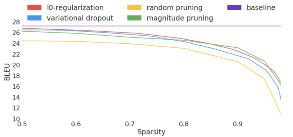
Mainly, pruning acts as an architecture search within the network. In fact, at low levels of sparsity (~40%), a model will typically generalize slightly better, as pruning acts as a regularizer. At higher levels, the pruned model will match the baseline. Pushing it further, the model will begin to generalize worse than the baseline, but with better performance. For example, a well-pruned ResNet-50 model can nearly match the baseline accuracy on ImageNet at 90% sparsity (90% of the weights in the model are zero).
At the extremes, the sparsity vs. accuracy tradeoff is an excellent addition to the data scientist’s toolset. Instead of spending significant amounts of time searching and training multiple networks to meet the desired deployment criteria– such as using MobileNet over ResNet – a high accuracy model can be adjusted using sparsity to meet performance/deployment criteria. In fact, scaling up the model size by adding more channels or layers and then pruning will have net positive results on the accuracy vs. performance tradeoff curve, compared to the pruned baseline.
Pruning Algorithms
Given the recent, renewed interest in pruning, many algorithms have been developed in the research community to prune models to higher sparsity levels, while preserving accuracy. A non-exhaustive list includes:
- Variational dropout
- Regularization methods such as L0 or Hoyer
- Second-order methods as in Lecun’s original pruning paper or the WoodFisher approach
- Weight reintroduction techniques such as RigL
- And gradual magnitude pruning (GMP).
Comparisons between the existing methods vary, and unfortunately, most papers lack direct and controlled comparisons. Several papers analyzing the current state of pruning techniques have appeared from Google and MIT to address this lack of control. The net results list GMP as the clear favorite. It either beats other approaches outright or matches more complicated methods close enough so that the extra cost and complexity are not justified.

Our research has found GMP to be one of the best approaches to use due to its simplicity, ease of use, and performance on a wide variety of models. Additionally, GMP allows for very fine control over the model’s sparsity distribution, something that’s lacking from most other methods. This control guarantees that after pruning a model, it will have the desired performance characteristics. Finally, using GMP with intelligently selected sparsity distributions for the model can far exceed other algorithms.
Structured vs. Unstructured Pruning
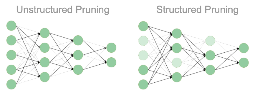
Most of the algorithms listed above can be formulated to support structured or unstructured pruning, but by default, results are generally reported using unstructured. The difference between the two comes from whether individual weights or groups of weights are removed together. This difference has not only performance implications but also affects the maximum achievable sparsity.

For unstructured pruning, individual weight connections are removed from a network by setting them to 0. Pruning, therefore, has the effect of introducing multiplications by 0 into the network, which can be turned into no-ops at prediction time. Because of this, software like the Neural Magic Inference Engine runs pruned networks much faster. Additionally, the model files can be stored compressed on disk, taking up much less space.
For structured pruning, groups of weight connections are removed together, such as entire channels or filters. Thus, structured pruning has the effect of changing the input and output shapes of layers and weight matrices. Because of this, nearly every system can successfully run structurally pruned networks faster. Unfortunately, structured pruning severely limits the maximum sparsity that can be imposed on a network when compared with unstructured pruning, therefore, severely limiting both the performance and memory improvements.
From a practical point of view, the reason for this difference is that pruning groups of weights and even whole channels takes away flexibility. Necessary connections in channels will have to be pruned away along with unimportant ones. From a loose theoretical point of view, when pruning channels or filters, the width of the layer (and overall network) is reduced, pushing the network further away from the universal approximation theorem and a gaussian approximation. Thus, we strongly recommend using unstructured whenever possible to better guarantee the quality of the model for performance and accuracy.
Learn More About Pruning
In our second post in the series, we will get into more depth on GMP. If you have questions or would like us to help you to speed up your neural networks with pruning, reach out to us!
About the author: Mark Kurtz is the Machine Learning Lead at Neural Magic. He’s an experienced software and machine learning leader with a demonstrated success in making machine learning models successful and performant. Mark manages teams and efforts that ensure organizations realize high returns from their machine learning investments. He is currently building a “software AI” engine at Neural Magic, with a goal to bring GPU-class performance for deep learning to commodity CPUs.


