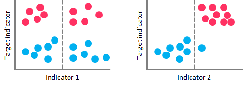
Now you may ask yourself: how do DTs know which features to select and how to split the data? To understand that, we need to get into some details.
All DTs perform basically the same task: they examine all the attributes of the dataset to find the ones that give the best possible result by splitting the data into subgroups. They perform this task recursively by splitting subgroups into smaller and smaller units until the Tree is finished (stopped by certain criteria).
This decision of making splits heavily affects the Tree’s accuracy and performance, and for that decision, DTs can use different algorithms that differ in the possible structure of the Tree (e.g. the number of splits per node), the criteria on how to perform the splits, and when to stop splitting.
So, how can we define which attributes to split, when and how to split them? To answer this question, we must review the main DTs algorithms:
CHAID
The Chi-squared Automatic Interaction Detection (CHAID) is one of the oldest DT algorithms methods that produces multiway DTs (splits can have more than two branches) suitable for classification and regression tasks. When building Classification Trees (where the dependent variable is categorical in nature), CHAID relies on the Chi-square independence tests to determine the best split at each step. Chi-square tests check if there is a relationship between two variables, and are applied at each stage of the DT to ensure that each branch is significantly associated with a statistically significant predictor of the response variable.
In other words, it chooses the independent variable that has the strongest interaction with the dependent variable.
Additionally, categories of each predictor are merged if they are not significantly different between each other, with respect to the dependent variable. In the case of Regression Trees (where the dependent variable is continuous), CHAID relies on F-tests (instead of Chi-square tests) to calculate the difference between two population means. If the F-test is significant, a new partition (child node) is created (which means that the partition is statistically different from the parent node). On the other hand, if the result of the F-test between target means is not significant, the categories are merged into a single node.
CHAID does not replace missing values and handles them as a single class which may merge with another class if appropriate. It also produces DTs that tend to be wider rather than deeper (multiway characteristic), which may be unrealistically short and hard to relate to real business conditions. Additionally, it has no pruning function.
Although not the most powerful (in terms of detecting the smallest possible differences) or fastest DT algorithm out there, CHAID is easy to manage, flexible and can be very useful.
You can find an implementation of CHAID with R in this link
CART
CART is a DT algorithm that produces binary Classification or regression trees, depending on whether the dependent (or target) variable is categorical or numeric, respectively. It handles data in its raw form (no preprocessing needed), and can use the same variables more than once in different parts of the same DT, which may uncover complex interdependencies between sets of variables.
In the case of Classification Trees, CART algorithm uses a metric called Gini Impurity to create decision points for classification tasks. Gini Impurity gives an idea of how fine a split is (a measure of a node’s “purity”), by how mixed the classes are in the two groups created by the split. When all observations belong to the same label, there’s a perfect classification and a Gini Impurity value of 0 (minimum value). On the other hand, when all observations are equally distributed among different labels, we face the worst case split result and a Gini Impurity value of 1 (maximum value).
In the case of Regression Trees, CART algorithm looks for splits that minimize the Least Square Deviation (LSD), choosing the partitions that minimize the result over all possible options. The LSD (sometimes referred to as “variance reduction”) metric minimizes the sum of the squared distances (or deviations) between the observed values and the predicted values. The difference between the predicted and observed values is called “residual”, which means that LSD chooses the parameter estimates so that the sum of the squared residuals is minimized.
LSD is well suited for metric data and has the ability to correctly capture more information about the quality of the split than other algorithms.
The idea behind CART algorithm is to produce a sequence of DTs, each of which is a candidate to be the “optimal Tree”. This optimal Tree is identified by evaluating the performance of every Tree through testing (using new data, which the DT has never seen before) or performing cross-validation(dividing the dataset into “k” number of folds, and perform testings on each fold).
CART doesn’t use an internal performance measure for Tree selection. Instead, DTs performances are always measured through testing or via cross-validation, and the Tree selection proceeds only after this evaluation has been done.
ID3
The Iterative Dichotomiser 3 (ID3) is a DT algorithm that is mainly used to produce Classification Trees. Since it hasn’t proved to be so effective building Regression Trees in its raw data, ID3 is mostly used for classification tasks (although some techniques such as building numerical intervals can improve its performance on Regression Trees).
ID3 splits data attributes (dichotomizes) to find the most dominant features, performing this process iteratively to select the DT nodes in a top-down approach.
For the splitting process, ID3 uses the Information Gain metric to select the most useful attributes for classification. Information Gain is a concept extracted from Information Theory, that refers to the decrease in the level of randomness in a set of data: basically, it measures how much “information” a feature gives us about a class. ID3 will always try to maximize this metric, which means that the attribute with the highest Information Gain will split first.
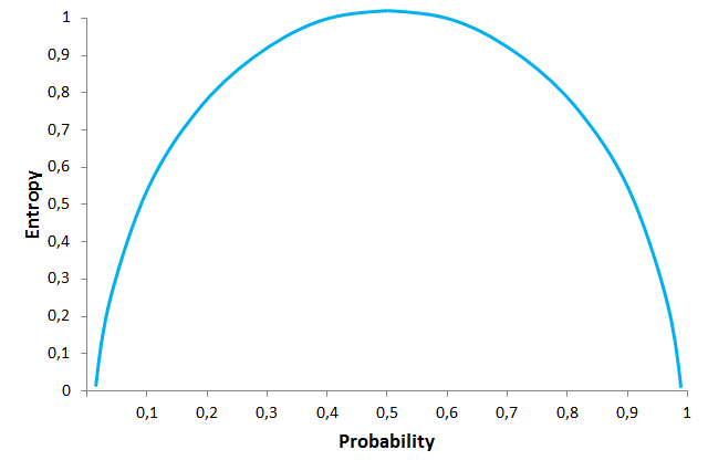
Information Gain is directly linked to the concept of Entropy, which is the measure of the amount of uncertainty or randomness in the data. Entropy values range from 0 (when all members belong to the same class or the sample is completely homogeneous) to 1 (when there is perfect randomness or unpredictability, or the sample is equally divided).
You can think it this way: if you want to make an unbiased coin toss, there is complete randomness or an Entropy value of 1 (“heads” and “tails” are equally like, with a probability of 0.5 each). On the other hand, if you make a coin toss, with for example a coin that has “tails” on both sides, randomness is removed from the event and the Entropy value is 0 (probability of getting “tails” will jump to 1, and probability of “heads” will drop to 0).
This is important because Information Gain is the decrease in Entropy, and the attribute that yields the largest Information Gain is chosen for the DT node.
But ID3 has some disadvantages: it can’t handle numeric attributes nor missing values, which can represent serious limitations.
C4.5
C4.5 is the successor of ID3 and represents an improvement in several aspects. C4.5 can handle both continuous and categorical data, making it suitable to generate Regression and Classification Trees. Additionally, it can deal with missing values by ignoring instances that include non-existing data.
Unlike ID3 (which uses Information Gain as splitting criteria), C4.5 uses Gain Ratio for its splitting process. Gain Ratio is a modification of the Information Gain concept that reduces the bias on DTs with huge amount of branches, by taking into account the number and size of the branches when choosing an attribute. Since Information Gain shows an unfair favoritism towards attributes with many outcomes, Gain Ratio corrects this trend by considering the intrinsic information of each split (it basically “normalizes” the Information Gain by using a split information value). This way, the attribute with the maximum Gain Ratio is selected as the splitting attribute.
Additionally, C4.5 includes a technique called windowing, which was originally developed to overcome the memory limitations of earlier computers. Windowing means that the algorithm randomly selects a subset of the training data (called a “window”) and builds a DT from that selection. This DT is then used to classify the remaining training data, and if it performs a correct classification, the DT is finished. Otherwise, all the misclassified data points are added to the windows, and the cycle repeats until every instance in the training set is correctly classified by the current DT. This technique generally results in DTs that are more accurate than those produced by the standard process due to the use of randomization, since it captures all the “rare” instances together with sufficient “ordinary” cases.
Another capability of C4.5 is that it can prune DTs.
C4.5’s pruning method is based on estimating the error rate of every internal node, and replacing it with a leaf node if the estimated error of the leaf is lower. In simple terms, if the algorithm estimates that the DT will be more accurate if the “children” of a node are deleted and that node is made a leaf node, then C4.5 will delete those children.
The latest version of this algorithm is called C5.0, which was released under a proprietary license and presents some improvements over C4.5 like:
-Improved speed: C5.0 is significantly faster than C4.5 (by several orders of magnitude).
-Memory usage: C5.0 is more memory efficient than C4.5.
-Variable misclassification costs: in C4.5 all errors are treated as equal, but in practical applications, some classification errors are more serious than others. C5.0 allows defining separate cost for each predicted/actual class pair.
-Smaller decision trees: C5.0 gets similar results to C4.5 with considerably smaller DTs.
-Additional data types: C5.0 can work with dates, times, and allows values to be noted as “not applicable.”
-Winnowing: C5.0 can automatically winnow the attributes before a classifier is constructed, discarding those that may be unhelpful or seem irrelevant.
You can find a comparison between C4.5 and C5.0 here
The dark side of the Tree
Surely DTs have lots of advantages. Because of their simplicity and the fact that they are easy to understand and implement, they are widely used for different solutions in a large number of industries. But you also need to be aware of its disadvantages.
DTs tend to overfit on their training data, making them perform badly if data previously shown to them doesn’t match to what they are shown later.
They also suffer from high variance, which means that a small change in the data can result in a very different set of splits, making interpretation somewhat complex. They suffer from an inherent instability, since due to their hierarchical nature, the effect of an error in the top splits propagate down to all of the splits below.
In Classification Trees, the consequences of misclassifying observations are more serious in some classes than others. For example, it is probably worse to predict that a person will not have a heart attack when he/she actually will, than vice versa. This problem is mitigated in algorithms like C5.0, but remains a serious issue in others.
DTs can also create biased Trees if some classes dominate over others. This is a problem in unbalanced datasets (where different classes in the dataset have a different number of observations), in which case it is recommended to balance de dataset prior to building the DT.
In the case of Regression Trees, DTs can only predict within the range of values they created based on the data they saw before, which means that they have boundaries on the values they can produce.
At each level, DTs look for the best possible split so that they optimize the corresponding splitting criteria.
But DTs splitting algorithms can’t see far beyond the current level in which they are operating (they are “greedy”), which means that they look for a locally optimal and not a globally optimal at each step.
DTs algorithms grow Trees one node at a time according to some splitting criteria and don’t implement any backtracking technique.
The power of the crowd in a guide to decision trees
But here are the good news: there are different strategies to overcome these drawbacks. Ensemble methods combine several DTs to improve the performance of single DTs, and are a great resource to get over the problems already described. The idea is to train multiple models using the same learning algorithm to achieve superior results.
Probably the 2 most common techniques to perform ensemble DTs are Bagging and Boosting.
Bagging (or Bootstrap Aggregation) is used when the goal is to reduce the variance of a DT. Variance relates to the fact that DTs can be quite unstable because small variations in the data might result in a completely different Tree being generated. So, the idea of Bagging is to solve this issue by creating in parallel random subsets of data (from the training data), where any observation has the same probability to appear in a new subset data. Next, each collection of subset data is used to train DTs, resulting in an ensemble of different DTs. Finally, an average of all predictions of those different DTs is used, which produces a more robust performance than single DTs. Random Forest is an extension over Bagging, which takes one extra step: in addition to taking the random subset of data, it also takes a random selection of features rather than using all features to grow DTs.
Boosting is another technique that creates a collection of predictors to reduce the variance of a DT, but with a different approach. It uses a sequential method where it fits consecutive DTS, and at every step, tries to reduce the errors from the prior Tree. With Boosting techniques, each classifier is trained on data, taking into account the previous classifier success. After each training step, the weights are redistributed based on the previous performance. This way, misclassified data increases its weights to emphasize the most difficult cases, so that subsequent DTs will focus on them during their training stage and improve their accuracy. Unlike Bagging, in Boosting the observations are weighted and therefore some of them will take part in the new subsets of data more often. As a result of this process, the combination of the whole sets improves the performance of DTs.
Within Boosting, there are several alternatives to determine the weights to use in the training and classification steps (e.g. Gradient Boost, XGBoost, AdaBoost, and others).
You can find a description of similarities and differences between both techniques here


