Introduction to Seq2Seq Models

Introduction

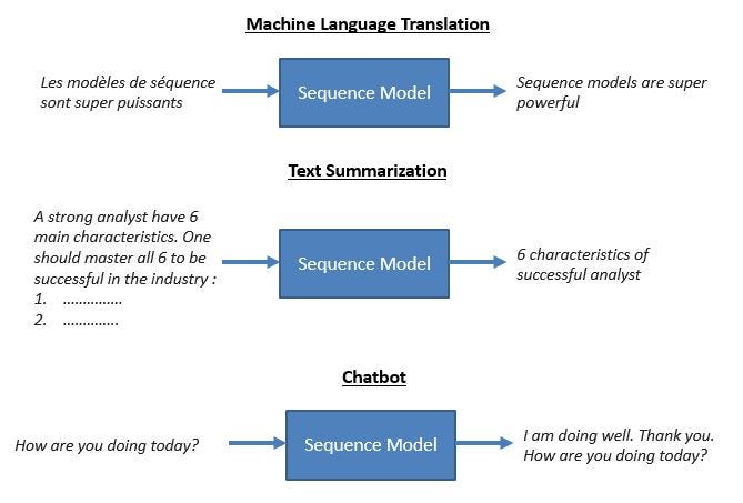
Sequence to Sequence (often abbreviated to seq2seq) models is a special class of Recurrent Neural Network architectures that we typically use (but not restricted) to solve complex Language problems like Machine Translation, Question Answering, creating Chatbots, Text Summarization, etc.

Overview

In this article, I would give you an overview of sequence to sequence models which became quite popular for different tasks like machine translation, video captioning, image captioning, question answering, etc.

Prerequisites: The reader should already be familiar with neural networks and, in particular, recurrent neural networks (RNNs). In addition, knowledge of LSTM or GRU models is preferable. If you are not familiar with LSTM I would prefer you to read LSTM- Long Short-Term Memory.

Use Cases of the Sequence to Sequence Models

Sequence to sequence models lies behind numerous systems that you face on a daily basis. For instance, seq2seq model powers applications like Google Translate, voice-enabled devices, and online chatbots. The following are some of the applications:

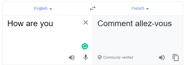
• Machine translation — a 2016 paper from Google shows how the seq2seq model’s translation quality “approaches or surpasses all currently published results”.

• Speech recognition — another Google paper that compares the existing seq2seq models on the speech recognition task.

These are only some applications where seq2seq is seen as the best solution. This model can be used as a solution to any sequence-based problem, especially ones where the inputs and outputs have different sizes and categories.

We will talk more about the model structure below.

Encoder-Decoder Architecture

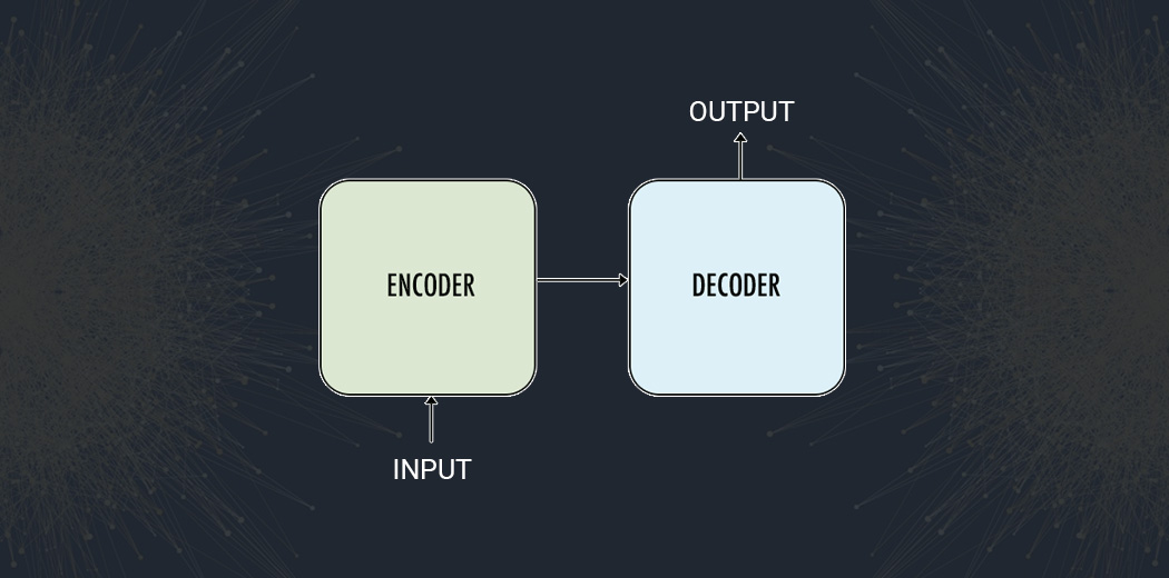
The most common architecture used to build Seq2Seq models is Encoder-Decoder architecture.

As the name implies, there are two components — an encoder and a decoder.

Encoder

• Both encoder and the decoder are LSTM models (or sometimes GRU models)
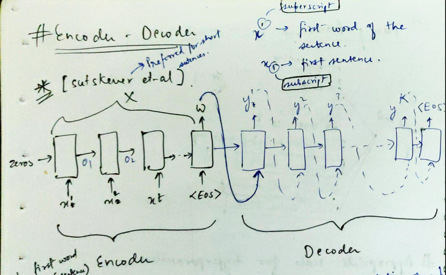
• Encoder reads the input sequence and summarizes the information in something called the internal state vectors or context vector (in case of LSTM these are called the hidden state and cell state vectors). We discard the outputs of the encoder and only preserve the internal states. This context vector aims to encapsulate the information for all input elements in order to help the decoder make accurate predictions.
• The hidden states h_i are computed using the formula:

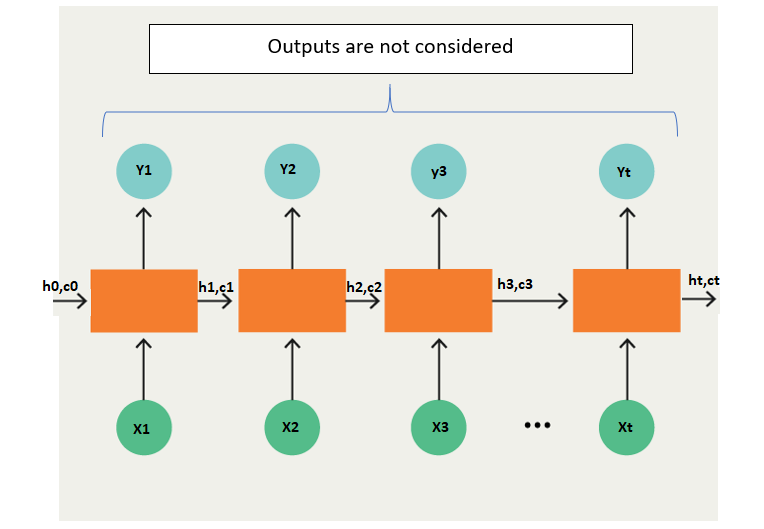
The LSTM reads the data, one sequence after the other. Thus if the input is a sequence of length ‘t’, we say that LSTM reads it in ‘t’ time steps.

1. Xi = Input sequence at time step i.

2. hi and ci = LSTM maintains two states (‘h’ for hidden state and ‘c’ for cell state) at each time step. Combined together these are internal state of the LSTM at time step i.

3. Yi = Output sequence at time step i. Yi is actually a probability distribution over the entire vocabulary which is generated by using a softmax activation. Thus each Yi is a vector of size “vocab_size” representing a probability distribution.

Decoder

• The decoder is an LSTM whose initial states are initialized to the final states of the Encoder LSTM, i.e. the context vector of the encoder’s final cell is input to the first cell of the decoder network. Using these initial states, the decoder starts generating the output sequence, and these outputs are also taken into consideration for future outputs.
• A stack of several LSTM units where each predicts an output y_t at a time step t.
• Each recurrent unit accepts a hidden state from the previous unit and produces and output as well as its own hidden state.
• Any hidden state h_i is computed using the formula:

• The output y_t at time step t is computed using the formula:

• We calculate the outputs using the hidden state at the current time step together with the respective weight W(S). Softmax is used to create a probability vector which will help us determine the final output (e.g. word in the question-answering problem).

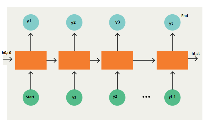
We will add two tokens in the output sequence as follows:

Example:

“START_ John is hard working _END”.

The most important point is that the initial states (h0, c0) of the decoder are set to the final states of the encoder. This intuitively means that the decoder is trained to start generating the output sequence depending on the information encoded by the encoder.

Finally, the loss is calculated on the predicted outputs from each time step and the errors are backpropagated through time in order to update the parameters of the network. Training the network over a longer period with a sufficiently large amount of data results in pretty good predictions.

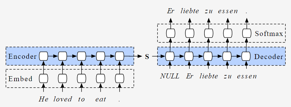
• During inference, we generate one word at a time.
• The initial states of the decoder are set to the final states of the encoder.
• The initial input to the decoder is always the START token.
• At each time step, we preserve the states of the decoder and set them as initial states for the next time step.
• At each time step, the predicted output is fed as input in the next time step.
• We break the loop when the decoder predicts the END token.

Drawbacks of Encoder-Decoder Models

There are two primary drawbacks to this architecture, both related to length.

1. Firstly, as with humans, this architecture has very limited memory. The ultimate hidden state of the LSTM, referred to as S or W, is tasked with encapsulating the entire sentence for translation. Typically, S or W comprises only a few hundred units (i.e., floating-point numbers). However, cramming too much into this fixed-dimensional vector leads to increased lossiness in the neural network. Thinking of neural networks in terms of the “lossy compression” they’re required to perform is sometimes quite useful.
2. Second, as a general rule of thumb, the deeper a neural network is, the harder it is to train. For recurrent neural networks, the longer the sequence is, the deeper the neural network is along the time dimension.This results in vanishing gradients, where the gradient signal from the objective that the recurrent neural network learns from disappears as it travels backward. Even with RNNs specifically made to help prevent vanishing gradients, such as the LSTM, this is still a fundamental problem.

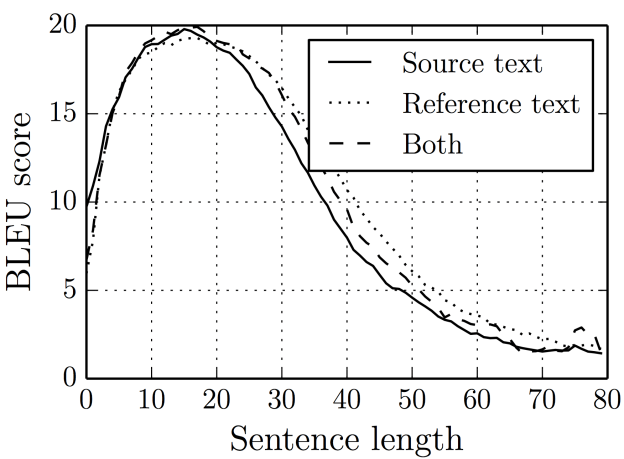
Furthermore, for more robust and lengthy sentences we have models like Attention Models and Transformers.

Here this is my GitHub repository for complete word level as well as character level encoder-decoder Model.

Conclusion

The document examines Sequence to Sequence models, their Encoder-Decoder architecture, and applications, while acknowledging their limitations, especially with long sequences. Despite drawbacks, such as struggles with lengthy sequences, their impact on fields like machine translation remains significant, underscoring the necessity for further research to boost efficiency.