Introduction
Decision Trees are probably one of the common machine learning algorithms and this is something every Data Science beginner should know before deep-diving into the advanced machine learning algorithms. And one of the important things is to understand the working of Decision Trees.
In this article, you’ll understand the basics of Decision Trees such as splitting, ideal split, and pure nodes.
Note: If you are more interested in learning concepts in an Audio-Visual format, We have this entire article explained in the video below. If not, you may continue reading.
So let’s begin! We’ll start off by using a very simple example.
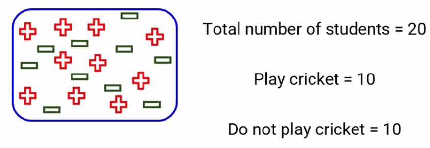
Let’s say we have data of 20 students, out of which 10 play cricket whereas 10 do not. So the red plus sign here represents the student who does play cricket and the green negative ones represent who does not play cricket.
Now we have the following features of the students
- Height- The height of the students
- Performance- Their performance in the class tells us how the students have been performing in the tests that are conducted in the class
- Class- Finally, we have their class which basically defines the current class of the student
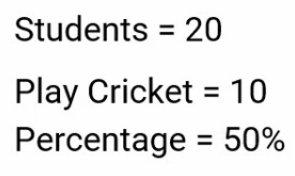
Using these features we want to train a model and predict whether they will play cricket or not. Now if we look at this data that is available to us, we have a total of 20 students out of which 10 play cricket and hence the percentage of students who do play cricket is 50%. And we have attributes of students like height, performance in the class and from which class they belong.
Now the teacher wants to identify the sub-groups. These sub-groups are very similar with respect to playing cricket or not based on the given attributes.
Decision Tree Split – Height
For example, let’s say we are dividing the population into subgroups based on their height. We can choose a height value, let’s say 5.5 feet, and split the entire population such that students below 5.5 feet are part of one sub-group and those above 5.5 feet will be in another subgroup. After splitting let’s say we got this distribution-
As you can see, there are 8 students who are below 5.5 feet and out of those 8 students, only 2 are actually playing Cricket. Hence the percentage of students below 5.5 feet in height and play cricket is 25% percent. And we can say that 75% time people who are below 5.5 feet do not play cricket. Whereas there 12 students above 5.5 feet and out of those 12 students 8 are playing cricket. And the percentage of playing Cricket, in this case, is somewhere around 67%.
At a broad level, the teacher would be more confident while selecting students from these two groups, compared to our original population.
What do you think, out of the given three variables height is the right one, and why 5.5 feet? Could it be 6 feet or something else as well?
Decision Tree Split – Performance
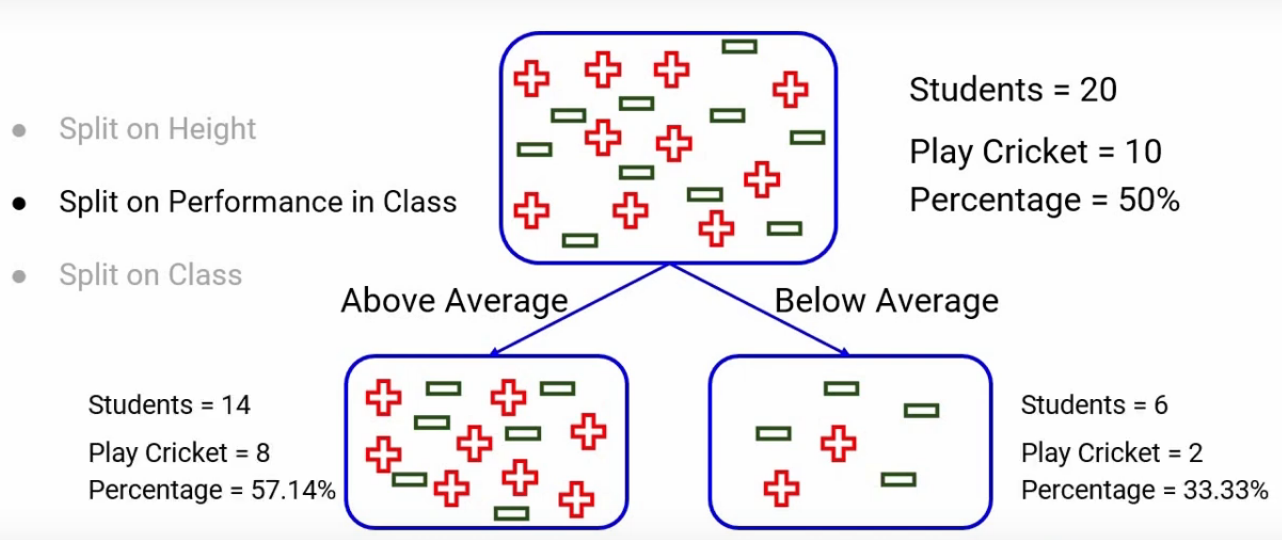
Let’s first try with another variable. Let’s split the population-based on performance. Here the performance is defined as either Above average or Below average. We will again divide the population based on these categories and let’s say we got a distribution like this-
Here, 14 students are above average, and out of these 14 students 8 play cricket and the percentage will be somewhere around 57%. In the below-average category, we have a total of 6 students, out of which 2 play cricket and the percentage will be, you guessed it, around 33%.
Decision Tree Split – Class
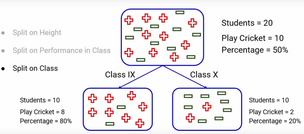
Finally, we have one more variable, Class and hence we can split the entire data on the class as well. Let’s say the students in this data are either from class 9 or class 10 and hence we can use them as categories to split the data. After the split, we get this distribution-
A lot of students in class 9 play cricket whereas the number becomes quite less if you look at class 10. Perhaps students in class 10 are busy with their board exams or there could be a lot of reasons. Let’s look at the numbers and percentages, in our data, there are 10 students from class 9 and 10 from class 10. In class 9, 8 out of 10 are playing cricket which is exactly 80% whereas in class 10 only 2 are playing cricket which comes out to be 20%.
This is how we can split the data based on the features available to us. If you would have noticed we have created three different decision trees till now. Every time we split the entire data into two subsets based on certain conditions or decisions and that’s how we got a decision tree.
As you have seen we have three decision trees so far, which of these three decision trees do you think is better? or we can say which is giving more confidence to the teacher while predicting the behavior of students whether they play cricket or not. In decision trees, what we want is to have a decision that can separate the classes, which in our case is- whether the student plays or does not play cricket. So we want all the positives to be on one side or one node and all the negatives on the other node.
Which of these three scenarios do you think is the best split, just think about it for a second before we move on. Okay, if you look at the split on class in the third decision tree, it has segregated 80% of students who play cricket which is more than any of the other two splits. So we can say that the split on class is better in the other splits as it has produced almost pure nodes.
What is an Ideal Split in Decision Trees?
Can you guess what would have been an ideal split?
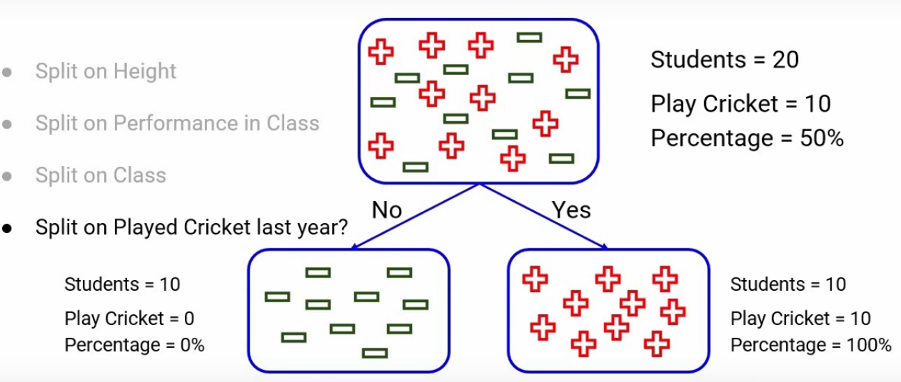
An ideal split would be the one that can segregate the positives in this case completely from the negatives and that would have produced the purest nodes.
Considered one more feature of the students which tells whether the student played cricket last year or not. Let’s say we split the entire data based on this feature. There will be two categories Yes and No. Generally, students who played cricket last year have higher chances of playing cricket this year as well, and hence after the split, we get this distribution-
You can see it has separated all the positives from all the negatives and when you look at the percentages, there are 10 students who did not play cricket last year and out of those 10 none played cricket this year as well and hence the percentage there is 0%. Similarly out of 10 students who played cricket last year, all of them played cricket this year as well and that is why this percentage is a full 100%.
A 100% pure node is a node that contains the data from a single class only.
Remember this is the ideal case, in practical real-world scenarios we have very less likely to have such features that can give you the completely pure nodes after the split. So if we look at the objective of decision trees, it is essential to have pure nodes.
We saw that the split on class produced the purest nodes out of all the other splits and that’s why we chose it as the first split. But the decision tree doesn’t stop there, we can have more splits as well. For example, we can split the class 9 node even further let’s say based on their heights or we can split the class 10 node based on the performance of students in that particular node.
The idea here is that we can have multiple splits and multiple decisions in a decision tree.
End Notes
We covered the basics of how to split Decision Trees so far. But the questions which you might be having right now is how we decide which split is better or what should be the first split or second split and so on. And how do you decide that what should be the sequence in which the split should be made? These are excellent questions and there are techniques to decide the purity of nodes based on which we can decide the best splitting point.
To understand decision trees in more depth, you can read the following article-
Don’t get confused, we’ll cover all these questions in our next article.


