This article was published as a part of the Data Science Blogathon
Introduction
In this article, I am gonna discuss various algorithms of image feature detection, description, and feature matching using OpenCV.
First of all, let’s see what is computer vision because OpenCV is an Open source Computer Vision library.
What happens when a human sees this image?

He will be able to recognize the faces which are there inside the images. So, in a simple form, computer vision is what allows computers to see and process visual data just like humans. Computer vision involves analyzing images to produce useful information.
What is a feature?
When you see a mango image, how can you identify it as a mango?
By analyzing the color, shape, and texture you can say that it is a mango.
The clues which are used to identify or recognize an image are called features of an image. In the same way, computer functions, to detect various features in an image.
We will discuss some of the algorithms of the OpenCV library that are used to detect features.
1. Feature Detection Algorithms
1.1 Harris Corner Detection
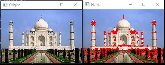
Harris corner detection algorithm is used to detect corners in an input image. This algorithm has three main steps.
- Determine which part of the image has a large variation in intensity as corners have large variations in intensities. It does this by moving a sliding window throughout the image.
- For each window identified, compute a score value R.
- Apply threshold to the score and mark the corners.
Here is the Python implementation of this algorithm.
import cv2
import numpy as np
imput_img = 'det_1.jpg'
ori = cv2.imread(imput_img)
image = cv2.imread(imput_img)
gray = cv2.cvtColor(image,cv2.COLOR_BGR2GRAY)
gray = np.float32(gray)
dst = cv2.cornerHarris(gray,2,3,0.04)
dst = cv2.dilate(dst,None)
image[dst>0.01*dst.max()]=[0,0,255]
cv2.imshow('Original',ori)
cv2.imshow('Harris',image)
if cv2.waitKey(0) & 0xff == 27:
    cv2.destroyAllWindows()
Here is the output.
1.2 Shi-Tomasi Corner Detector
This is another corner detection algorithm. It works similar to Harris Corner detection. The only difference here is the computation of the value of R. This algorithm also allows us to find the best n corners in an image.
Let’s see the Python implementation.
import numpy as np
import cv2
from matplotlib import pyplot as plt
img = cv2.imread('det_1.jpg')
ori = cv2.imread('det_1.jpg')
gray = cv2.cvtColor(img,cv2.COLOR_BGR2GRAY)
corners = cv2.goodFeaturesToTrack(gray,20,0.01,10)
corners = np.int0(corners)
for i in corners:
    x,y = i.ravel()
    cv2.circle(img,(x,y),3,255,-1)
cv2.imshow('Original', ori)
cv2.imshow('Shi-Tomasi', img)
cv2.waitKey(0)
cv2.destroyAllWindows()
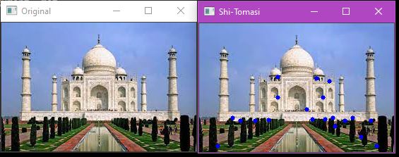
This is the output of the Shi-Tomasi algorithm. Here the top 20 corners are detected.
The next one is Scale-Invariant Feature Transform.
1.3 Scale-Invariant Feature Transform (SIFT)
SIFT is used to detect corners, blobs, circles, and so on. It is also used for scaling an image.

Consider these three images. Though they differ in color, rotation, and angle, you know that these are the three different images of mangoes. How can a computer be able to identify this?
Both Harris corner detection and Shi-Tomasi corner detection algorithms fail in this case. But SIFT algorithm plays a vital role here. It can detect features from the image irrespective of its size and orientation.
Let’s implement this algorithm.
import numpy as np
import cv2 as cv
ori = cv.imread('det_1.jpg')
img = cv.imread('det_1.jpg')
gray = cv.cvtColor(img,cv.COLOR_BGR2GRAY)
sift = cv.SIFT_create()
kp, des = sift.detectAndCompute(gray,None)
img=cv.drawKeypoints(gray,kp,img,flags=cv.DRAW_MATCHES_FLAGS_DRAW_RICH_KEYPOINTS)
cv.imshow('Original',ori)
cv.imshow('SIFT',image)
if cv.waitKey(0) & 0xff == 27:
    cv.destroyAllWindows()
The output is shown below.
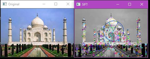
You can see that there are some lines and circles in the image. The size and orientation of the feature are indicated by the circle and line inside the circle respectively.
We will see the next algorithm of feature detection.
1.4 Speeded-up Robust Features (SURF)
SURF algorithm is simply an upgraded version of SIFT.
Let’s implement this.
import numpy as np
import cv2 as cv
ori =cv.imread('/content/det1.jpg')
img = cv.imread('/content/det1.jpg')
surf = cv.xfeatures2d.SURF_create(400)
kp, des = surf.detectAndCompute(img,None)
img2 = cv.drawKeypoints(img,kp,None,(255,0,0),4)
cv.imshow('Original', ori)
cv.imshow('SURF', img2)
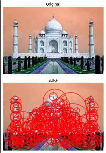
Next, we will see how to extract another feature called bob.
2. Detection of blobs
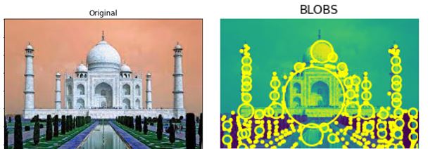
BLOB stands for Binary Large Object. It refers to a group of connected pixels or regions in a particular binary image that shares a common property. These regions are contours in OpenCV with some extra features like centroid, color, area, a mean, and standard deviation of the pixel values in the covered region. Let’s
implement this one.
import cv2
import numpy as np;
ori = cv2.imread('det_1.jpg')
im = cv2.imread("det_1.jpg", cv2.IMREAD_GRAYSCALE)
detector = cv2.SimpleBlobDetector_create()
keypoints = detector.detect(im)
im_with_keypoints = cv2.drawKeypoints(im, keypoints, np.array([]), (0,0,255), cv2.DRAW_MATCHES_FLAGS_DRAW_RICH_KEYPOINTS)
cv2.imshow('Original',ori)
cv2.imshow('BLOB',im_with_keypoints)
if cv2.waitKey(0) & 0xff == 27:
    cv2.destroyAllWindows()
Let’s see the output. Here, the blobs are detected very well.
Now, let’s jump into feature descriptor algorithms.
3. Feature Descriptor Algorithms
Features are typically distinct points in an image and the descriptor gives a signature, so it describes the key point that is considered. It extracts the local neighborhood around that point so a local image patch is created and a signature from this local patch is computed.
3.1 Histogram of Oriented Gradients (HoG)
Before the advent of deep learning, HoG was one of the most prominent feature descriptors for object
detection applications. HoG is a technique that is used to count the occurrence of gradient orientation in localized portions of an image.
Let’s implement this algorithm.
from skimage.feature import hog
import cv2
ori = cv2.imread('/content/det1.jpg')
img = cv2.imread("/content/det1.jpg")
_, hog_image = hog(img, orientations=8, pixels_per_cell=(16, 16),
                    cells_per_block=(1, 1), visualize=True, multichannel=True)
cv2.imshow('Original', ori)
cv2.imshow('HoG', hog_image)
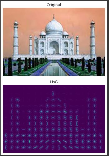
The next one is BRIEF.
3.2 Binary Robust Independent Elementary Features (BRIEF)
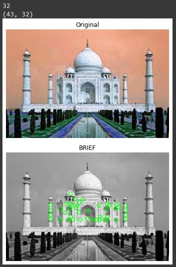
BRIEF is an alternative to the popular SIFT descriptor and they are faster to compute and more compact.
Let’s see its implementation.
import numpy as np
import cv2 as cv
ori = cv.imread('/content/det1.jpg')
img = cv.imread('/content/det1.jpg',0)
star = cv.xfeatures2d.StarDetector_create()
brief = cv.xfeatures2d.BriefDescriptorExtractor_create()
kp = star.detect(img,None)
kp, des = brief.compute(img, kp)
print( brief.descriptorSize() )
print( des.shape )
img2 = cv.drawKeypoints(img, kp, None, color=(0, 255, 0), flags=0)
cv.imshow('Original', ori)
cv.imshow('BRIEF', img2)
Here is the result.
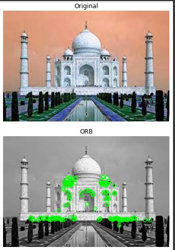
3.3 Oriented FAST and Rotated BRIEF (ORB)
ORB is a one-shot facial recognition algorithm. It is currently being used in your mobile phones and apps like Google photos in which you group the people stab you see the images are grouped according to the people. This algorithm does not require any kind of major computations. It does not require GPU. Here, two algorithms are involved. FAST and BRIEF. It works on keypoint matching. Key point matching of distinctive regions in an image like the intensity variations.
Here is the implementation of this algorithm.
import numpy as np
import cv2
ori = cv2.imread('/content/det1.jpg')
img = cv2.imread('/content/det1.jpg', 0)
orb = cv2.ORB_create(nfeatures=200)
kp = orb.detect(img, None)
kp, des = orb.compute(img, kp)
img2 = cv2.drawKeypoints(img, kp, None, color=(0, 255, 0), flags=0)
cv2.imshow('Original', ori)
cv2.imshow('ORB', img2)
Here is the output.
Now, let’s see about feature matching.
4. Feature Matching
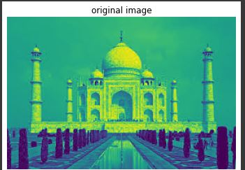
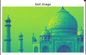
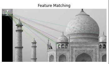
Feature matching is like comparing the features of two images which may be different in orientations, perspective, lightening, or even differ in sizes and colors. Let’s see its implementation.
import cv2
img1 = cv2.imread('/content/det1.jpg', 0)
img2 = cv2.imread('/content/88.jpg', 0)
orb = cv2.ORB_create(nfeatures=500)
kp1, des1 = orb.detectAndCompute(img1, None)
kp2, des2 = orb.detectAndCompute(img2, None)
bf = cv2.BFMatcher(cv2.NORM_HAMMING, crossCheck=True)
matches = bf.match(des1, des2)
matches = sorted(matches, key=lambda x: x.distance)
match_img = cv2.drawMatches(img1, kp1, img2, kp2, matches[:50], None)
cv2.imshow('original image', img1)
cv2.imshow('test image', img2)
cv2.imshow('Matches', match_img)
cv2.waitKey()
This is the result of this algorithm.
Endnotes
I hope you enjoyed this article. I have given a brief introduction to various feature detection, description, and feature matching techniques. The above-mentioned techniques are used in object detection, object tracking, and object classification applications.
The real fun starts when you start practicing. So, start practicing these algorithms, implement them in real-world projects, and see the fun. Keep learning.
The media shown in this article are not owned by Analytics Vidhya and are used at the Author’s discretion.


