Introduction
In the dynamic landscape of machine learning, synthesizing two potent techniques has given rise to a versatile model known as Adversarial Autoencoders (AAEs). Seamlessly blending the features of autoencoders and Generative Adversarial Networks (GANs), AAEs have emerged as a powerful tool for data generation, representation learning, and beyond. This article explores the essence of AAEs, their architecture, training process, and applications and provides a hands-on Python code example for an enriched understanding.

This article was published as a part of the Data Science Blogathon.
Table of contents
Understanding Autoencoders
Autoencoders, the foundation of AAEs, are neural network structures designed for data compression, dimensionality reduction, and feature extraction. The architecture consists of an encoder that maps input data into a latent space representation, followed by a decoder that reconstructs the original data from this reduced representation. Autoencoders have been instrumental in various fields, including image denoising, anomaly detection, and latent space visualization.
Autoencoders, a fundamental class of neural networks, can extract meaningful features from data while enabling efficient dimensionality reduction. Comprising two main components, an encoder compresses input data into a lower-dimensional latent representation, while the decoder reconstructs the original input from this compressed form. Autoencoders serve various purposes, including denoising, anomaly detection, and representation learning. Their capacity to capture essential data characteristics makes them a versatile tool for tasks across domains such as image processing, natural language processing, and more. By learning compact yet informative representations, autoencoders offer valuable insights into the underlying structures of complex datasets.

Introducing Adversarial Autoencoders
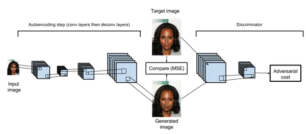
Adversarial Autoencoders (AAEs) are a remarkable fusion of autoencoders and Generative Adversarial Networks (GANs), innovatively combining their strengths. This hybrid model introduces an encoder-decoder architecture where the encoder maps input data into a latent space, and the decoder reconstructs it. The distinctive element of AAEs lies in integrating adversarial training, where a discriminator critiques the quality of generated data samples. This adversarial interaction between the generator and discriminator refines the latent space, fostering high-quality data generation.
AAEs find diverse applications in data synthesis, anomaly detection, and unsupervised learning, yielding robust latent representations. Their versatility offers promising avenues in various domains, such as image synthesis, text generation, etc. AAEs have garnered attention for their potential to enhance generative models and contribute to the advancement of artificial intelligence.
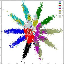
Adversarial Autoencoders, the result of integrating GANs with autoencoders, add an innovative dimension to generative modeling. By combining the latent space exploration of autoencoders with the adversarial training mechanism of GANs, AAEs balance the benefits of both worlds. This synergy results in enhanced data generation and more meaningful representations in the latent space.
AAE Architecture
The architectural blueprint of AAEs revolves around three pivotal components: the encoder, the generator, and the discriminator. The encoder condenses input data into a compressed representation in the latent space while the generator reconstructs the original data from these compressed representations. The discriminator introduces the adversarial aspect, aiming to differentiate between actual and generated data samples.
Training AAEs
The training of AAEs is an iterative dance of three players: the encoder, the generator, and the discriminator. The encoder and generator collaborate to minimize the reconstruction error, ensuring that the generated data resembles the original input. Concurrently, the discriminator hones its skills in distinguishing between real and generated data. This adversarial interaction leads to a refined latent space and improved data generation quality.
Applications of AAEs
The versatility of AAEs is exemplified through a spectrum of applications. AAEs shine in data generation tasks, capable of producing realistic samples in domains such as images, text, and more. Their anomaly detection prowess finds utility in identifying irregularities within datasets. Furthermore, AAEs are adept at unsupervised representation learning, aiding feature extraction and transfer learning.
Anomaly Detection and Data Denoising: AAEs’ latent space regularization empowers them to filter out noise and anomalies in data, rendering them a robust choice for data denoising and anomaly detection tasks.
Style Transfer and Data Transformation: By manipulating latent space vectors, AAEs enable style transfer between inputs, seamlessly morphing images and generating diverse versions of the same content.
Semi-Supervised Learning: AAEs can harness labeled and unlabeled data to improve supervised learning tasks, bridging the gap between supervised and unsupervised approaches.

Implementing an Adversarial Autoencoder
To provide a practical understanding of AAEs, let’s delve into a Python implementation using TensorFlow. In this example, we’ll focus on data denoising, showcasing how AAEs can excel in reconstructing clean data from noisy input.
(Note: Ensure you have TensorFlow and relevant dependencies installed before running the code below.)
import tensorflow as tf
from tensorflow.keras.layers import Input, Dense, Flatten, Reshape
from tensorflow.keras.models import Model
from tensorflow.keras.optimizers import Adam
from tensorflow.keras.losses import MeanSquaredError
from tensorflow.keras.datasets import mnist
import numpy as np

# Define the architecture of the Adversarial Autoencoder
def build_adversarial_autoencoder(input_dim, latent_dim):
    input_layer = Input(shape=(input_dim,))

    # Encoder
    encoder = Dense(128, activation='relu')(input_layer)
    encoder = Dense(latent_dim, activation='relu')(encoder)

    # Decoder
    decoder = Dense(128, activation='relu')(encoder)
    decoder = Dense(input_dim, activation='sigmoid')(decoder)

    # Build and compile the autoencoder
    autoencoder = Model(input_layer, decoder)
    autoencoder.compile(optimizer=Adam(), loss=MeanSquaredError())

    # Build and compile the adversary
    adversary = Model(input_layer, encoded)
    adversary.compile(optimizer=Adam(), loss='binary_crossentropy')

    return autoencoder, adversary

# Load and preprocess MNIST dataset
(input_train, _), (input_test, _) = mnist.load_data()
input_train = input_train.astype('float32') / 255.0
input_test = input_test.astype('float32') / 255.0
input_train = input_train.reshape((len(input_train), np.prod(input_train.shape[1:])))
input_test = input_test.reshape((len(input_test), np.prod(input_test.shape[1:])))

# Define AAE parameters
input_dim = 784
latent_dim = 32

# Build and compile the AAE
autoencoder, adversary = build_adversarial_autoencoder(input_dim, latent_dim)

# Train the AAE
autoencoder.fit(input_train, input_train,
                epochs=50,
                batch_size=256,
                shuffle=True,
                validation_data=(input_test, input_test))

# Generate denoised images
denoised_images = autoencoder.predict(input_test)
Hyperparameter Tuning
Hyperparameter tuning is critical to training any machine learning model, including Adversarial Autoencoders (AAEs). Hyperparameters are settings that determine the behavior of the model during training. Properly tuning these hyperparameters can greatly impact the generated samples’ convergence speed, stability, and quality. Some important hyperparameters include Learning Rate, Training Epochs, Batch size, Latent Dimension, Regularization Strength, etc. For simplicity, we will be tuning two hyperparameters here: number of training epochs and batch size.
# Hyperparameter Tuning
epochs = 50
batch_size = 256

# Train the AAE
autoencoder.fit(input_train, input_train,
                epochs=epochs,
                batch_size=batch_size,
                shuffle=True,
                validation_data=(input_test, input_test))

# Generate denoised images
denoised_images = autoencoder.predict(input_test)
Evaluation Metrics
Evaluating the quality of generated data from AAEs is crucial to ensure the model produces meaningful results. Here are a few evaluation metrics commonly used:
- Reconstruction Loss: This measures how well the generated samples can be reconstructed back to the original data. Lower reconstruction loss indicates better quality of generated samples.
- Inception Score: Inception Score measures the quality and diversity of generated images. It uses an auxiliary classifier trained on real data to evaluate the generated samples. Higher Inception Scores indicate better diversity and quality.
- Frechet Inception Distance (FID): FID calculates the distance between feature distributions of real and generated data in the Inception model’s feature space. Lower FID values indicate that the generated samples are closer to real data regarding statistics.
- Precision and Recall of Generated Data: Metrics from the field of information retrieval can also be applied to generated data. Precision measures the proportion of high quality generated samples, while recall measures the proportion of high-quality real samples that are successfully generated.
- Visual Inspection: While not a quantitative metric, visually inspecting the generated samples can provide insights into their quality and diversity.
# Evaluation Metrics
def compute_inception_score(images, inception_model, num_splits=10):
    scores = []
    splits = np.array_split(images, num_splits)
    for split in splits:
        split_scores = []
        for img in split:
            img = img.reshape((1, 28, 28, 1))
            img = np.repeat(img, 3, axis=-1)
            img = preprocess_input(img)
            pred = inception_model.predict(img)
            split_scores.append(pred)
        split_scores = np.vstack(split_scores)
        p_y = np.mean(split_scores, axis=0)
        kl_scores = split_scores * (np.log(split_scores) - np.log(p_y))
        kl_divergence = np.mean(np.sum(kl_scores, axis=1))
        inception_score = np.exp(kl_divergence)
        scores.append(inception_score)
    return np.mean(scores), np.std(scores)
Conclusion
As Generative AI continues to captivate researchers and practitioners alike, Adversarial Autoencoders emerge as distinct and versatile members of the generative family. By marrying the reconstruction prowess of autoencoders with the adversarial dynamics of GANs, AAEs navigate the delicate dance of data generation and latent space regularization. Their ability to denoise, transform styles, and harness the strength of labeled and unlabeled data renders them an essential toolset in the arsenal of creative AI. As this journey concludes, Adversarial Autoencoders beckon us to unlock new dimensions in generative AI and forge a path toward data synthesis that seamlessly marries control and innovation.
- Adversarial Autoencoders (AAEs) merge autoencoders and adversarial networks to reconstruct data and regularize the latent space.
- AAEs find applications in anomaly detection, data denoising, style transfer, and semi-supervised learning.
- The adversarial component in AAEs introduces a critic network that enforces latent space distribution adherence, balancing creativity and control.
- Implementation of AAEs requires a combination of deep learning concepts, adversarial training, and autoencoder architecture.
- Exploring the landscape of Adversarial Autoencoders provides a unique perspective on generative AI, opening doors to novel data transformation and regularization paradigms.
Frequently Asked Questions
A1: AAEs introduce adversarial training, enhancing their data generation capabilities and latent space representations.
A2: The discriminator in AAEs sharpens the latent space by distinguishing between genuine and generated data, fostering improved data generation.
A3: AAEs excel in anomaly detection, recognizing deviations from normal data patterns.
A4: Researchers have delved into conditional AAEs and domain-specific adaptations, tailoring AAEs to particular tasks.
The media shown in this article is not owned by Analytics Vidhya and is used at the Author’s discretion.


