This article was published as a part of the Data Science Blogathon.
Overview
· Markovian Assumption states that the past doesn’t give a piece of valuable information. Given the present, history is irrelevant to know what will happen in the future.
· Markov Chain is a stochastic process that follows the Markovian Assumption.
· Markov chain had given a new dimension to probability theory. The applicability can be seen almost in every field. Also, several value-able ideas have been developed with the basis of The Markov Chain; their importance is paramount in the field of data analytics.

Introduction
Being a student of Engineering, I often wondered how I used to pass in a few subjects after spending one week with them just before the final exam. Even after spending 3-4 hours per day, I could not unearth anything during the entire semester. My road to enlightenment for those subjects was a topsy-turvy journey until one week before the semester exam. I thought I’d fail. But from the final result, I used to think about how I have turned the tide within one week just before the exam?
A few years before, when I had started my journey in data analytics, I came across a theory, The Markov Chain. It gave the answer and the explanation that I was looking for in the prementioned scenario. One of the critical properties of the Markov Chain that caught my attention during that time was.
‘Only the most recent point in the trajectory affects what happens next.’
After this, I started to dig deep into the spiral of the Markov Chain. I’ll try to simplify the concept as much as I can with the help of real-life examples. I know the content itself is enormous and time-consuming to read. But you know what I have found while going through various materials. It’s full of some high-level mathematics. I feel from my learning experience that first, you need to have an intuition of the subject which comes from understanding which examples can give, followed by mathematics and then implementation via coding. This content is a mixture of more examples and a bit of Mathematics. I hope you will enjoy it.
Table Contents
· A Brief History
· Difference between Stochastic and Random Processes
· Importance of ‘Chain’ in Markov Chain
· Basics of Markov Chain
· Markovian and Non-Markovian Process
· Types of States in Markov Chain and concept of Random Walk
· Basics of Transition Matrix
· Hidden Markov Model
· Conclusion
· Reference of some advanced related topics and coding
· Coding Reference
· YouTube Links
· Used References
· Reference for Exercise and Solutions
· Reference for some Thought-Provoking Research Paper and Patents using Markov Chain
A Brief History on Markov Chain
More than a century ago, the Russian mathematician Andrei Andreevich Markov had discovered a complete novel branch of probability theory. Well, it has an exciting story. While going through Alexander Pushkin’s novel ‘Eugene Onegin,’ Markov spent hours sorting through patterns of vowels and consonants. On January 23, 1913, he addressed the Imperial Academy of Sciences in St. Petersburg with a synopsis of his finding. His findings did not alter the understanding or appreciation of Pushkin’s poem. Still, the technique he developed—now known as a Markov chain—extended probability theory in a new direction. Markov’s methodology went beyond coin-flipping and dice-rolling situations (where each event is independent of all others) to chains of linked events (where what happens next depends on the system’s current state).
Difference between Stochastic and Random Processes
So in a Markov chain, the future depends only upon the present, NOT upon the past. Let’s dig deep into it. As per Wikipedia, ‘A Markov chain or Markov process is a stochastic model which describes a sequence of possible events where the probability of each event depends only on the state attained in the previous event.’
For me, most of the time, we are confused with a word like Stochastic and Random. We often say ‘Stochastic means Random.’ But understanding the difference will help us comprehend the essence of the Markov Chain from a new perspective. Let me give you an example to explain it better. Let’s say I am at a pub and having a beer-drinking fun game with my friend. We have set out a rule. I’ll drink the number of bottles within a certain amount of time; my friend will drink exactly twice more than what I am drinking within that particular time. Like if I drink one bottle within one minute. He will drink two bottles within one minute. Or if I drink two bottles within one minute, he will drink four bottles within one minute and so on. I can define it like below :
|
1st event |
For me, bottle consumption : |
x |
|
Following Event |
For my friend, bottle consumption : |
2x |
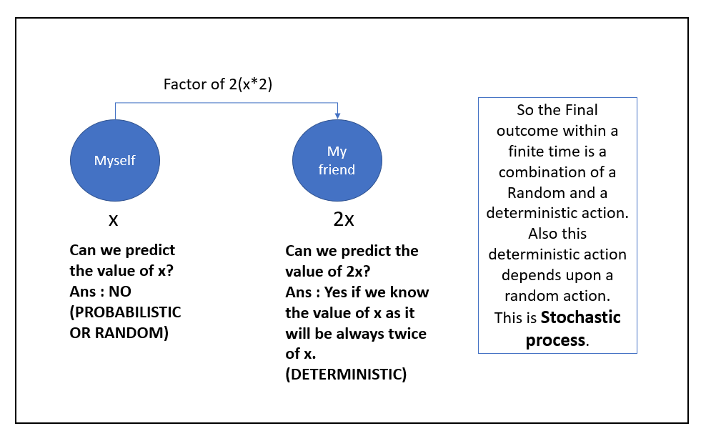
So Stochastic is not random. It is a combination of processes that must have at least a random process. And the deterministic process may or may not depend upon a random method. I hope I have cleared it. If you are confused about what a deterministic approach is, let me give you an example. The sun always rises in the east. It’s a deterministic statement, a universal truth. The sun will never rise in the west. Hey, but please don’t try the competition that I have mentioned before. Drinking is injurious to health. It’s a fictitious condition that I have mentioned.
Importance of ‘Chain’ in Markov Chain
One of the intrinsic philosophies of the Markov Chain is the realization of interconnectivity, which is quite an amusing factor for solving real-life problems. Folks who are familiar with the ‘Domino Effect ‘are aware that when you make a change of one behavioural attribute will activate a chain reaction and cause a shift in related behavioural attributes as well. Our Real-world is full of that examples. Please check the below examples.
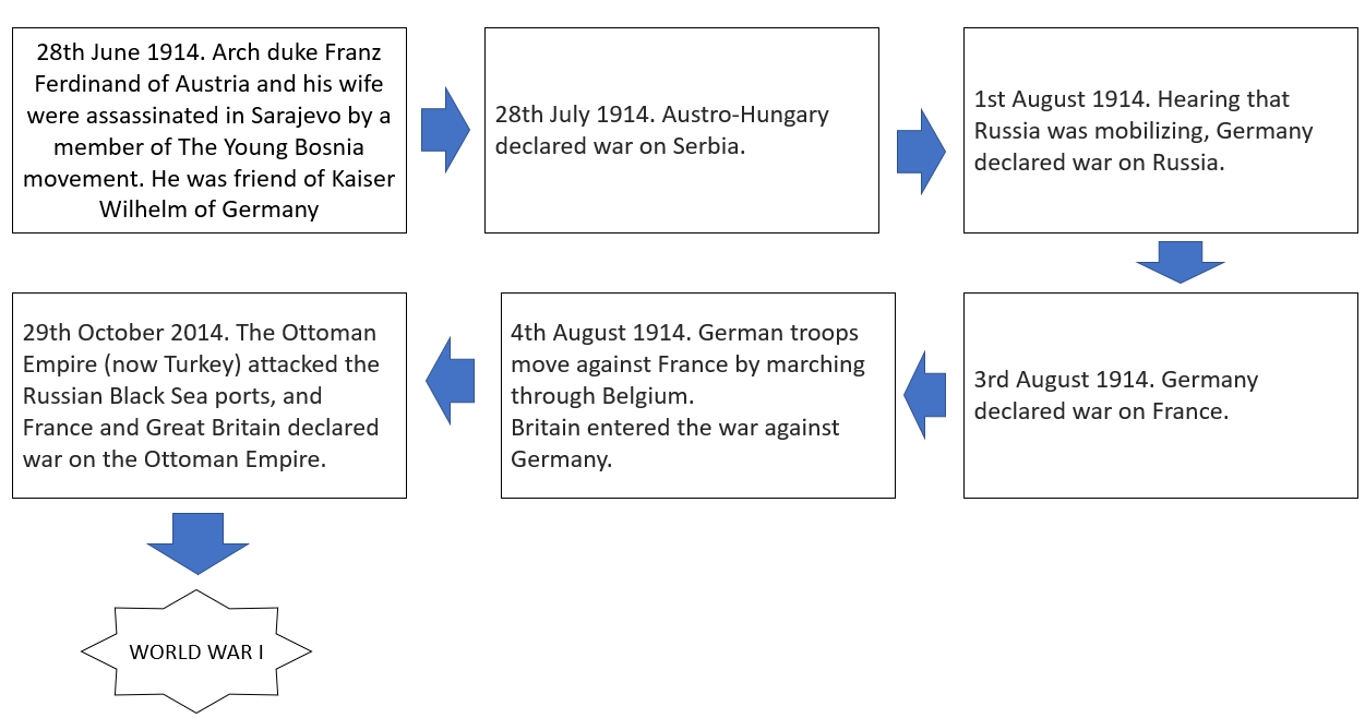
A series of chain reactions had developed an evil thing like world war I. Unfortunately Markov was still working on his research. Who knows, maybe if he could have come out with it in front of the world and if the world’s mathematician and statistician at that time used the Markov chain, we could have had a lesser impact that time. ‘Domino Effect’ is always happening in every sector like the stock market, Banking, IT, etc. As data scientists, our job is to reduce its effect. So we do that. The advent of computers and knowledge of ML and DL helped us avert the risk of a Stochastic system. And the first tool to start the journey was ‘The Markov Chain.’
Basics of Markov Chain
Now, let’s dig into some mathematical aspects. I’ll try to make it less tedious for you. It would be best if you had some
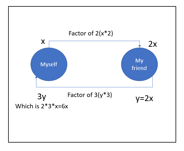
basic intuition of probability theory, linear algebra, and graph theory to understand it. Please don’t get scared. When we talk about a ‘Chain,’ we are getting an intuition of ‘Graph.’ Does the next question come if it’s cyclic or one-directional? Let me frame my previous beer-drinking example in a challenging competitive way. This time I have said to my friend, “The
the number of bottles of beer you are going to drink I’ll drink three times more than that” it’s a head-on challenge, right? Just check the below diagram to have better intuition. Below graphs shows in Markov chain basically, we can deal
with any graph.
Now let me give you an intuition about the recent past that governs the present outcome with my competitive pub gaming example. I am not going to explain it; observing the picture will be self-explanatory.
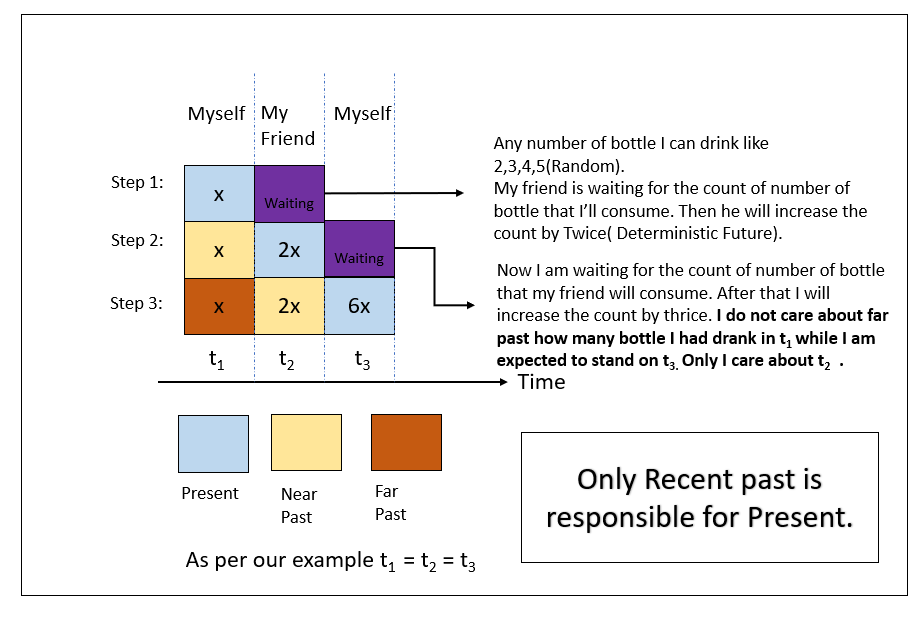
I hope the above depiction gives you some idea about the process. One thing you may be thinking Markov chain does not speak about any ‘Past.’ But why have I mentioned terms like ‘Near Past’ and ‘Far Past’? But I feel you can build a solid conceptual intuition by considering this. Just think ‘Near Past’ is ‘Yesterday’ and ‘Far Past’ starts from the day before ‘Yesterday’ believe me it will help you more. It is like Yesterday you have studied hard that is why Today you have a good result or like ‘Today’ you are motivated because ‘Yesterday’ you have met someone. I’ll give you another example from a real-life problem. Before that, let me define Markov Chain from a probabilistic point of view. Three elements determine a Markov chain.
· A state-space(S): If we define the seasonal states throughout a country, we can say, Summer, Monsoon, Autumn, Winter, Spring. So on Season State-space, we have prementioned five seasonal states.
· A Transition Operator(p(s(t+1))|p(s(t))) : It define probability of moving from s(t) to s(t+1). Like see below diagram.
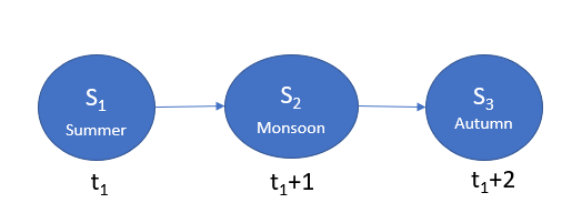
p(s(t1+1))|p(s(t1))=p(Monsoon)|p(Summer)
If the transition operator doesn’t change during the transition. The Markov chain is called ‘Time Homogenous.’ So if t1à∞ the chain will reach an equilibrium known as Stationary Distribution. For this the equation will look like below,
p(s(t1+1))|p(s(t1))= p(s(t1))|p(s(t1-1))
Now come to another example; you have seen that Gmail editor, while typing a mail, always suggests the next word. Most of the time, I have seen at least my case it’s right. Its an application of the Markov chain in the field of Natural Language Processing(NLP). More precisely, it uses the concept of’ n-gram.’ Our example is based on a bit of that. Consider the below three sentences.
Sentence 1: I am a Boy.
Sentence 2: I am a Girl.
Sentence 3: I am a Star.
Here we have considered the concept of uni-gram. I hope the below picture will give you the intuition of the n-gram concept.
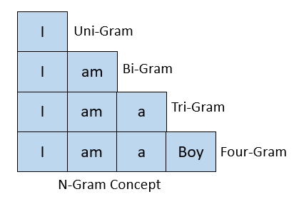
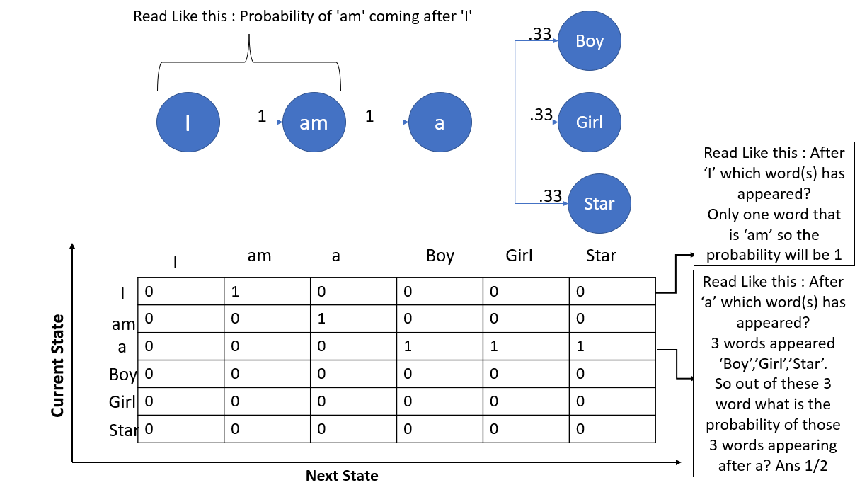
Let’s assume in The Markov chain we have processes X0, X1, X2, . . .. At time t, The state of a Markov chain is the value of Xt. The state-space(S) of a Markov chain is the set of values that each Xt can take. Like, S = {1, 2, 3, 4, 5, 6}.A specific set of values for X0, X1, X2. Known as the trajectory of a Markov chain is ‘Trajectory,’ synonymous with ‘path’ in a graph. For the sake of better understanding, consider State and Process as are same. So, Xi=Si. Let me also define the transition diagram of a Markov chain; it is a single weighted directed graph, where each vertex represents a state of the Markov chain, and there exist a directed edge which leads to vertex i(one state to another state or same state) from vertex j if the transition probability pij >0; this edge has the weight/probability of pij. Confused right? Just check the below diagram.
From the below transition diagram, we can see that our previous example has six states.
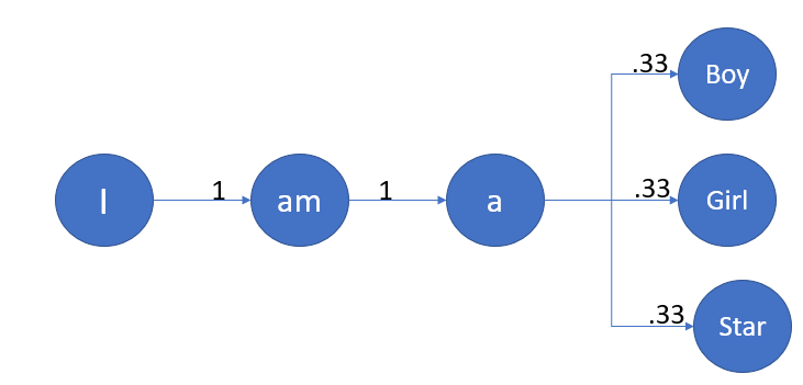
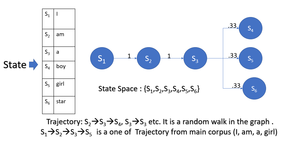
So one question may arise in your mind that how many states are possible. A theoretically infinite number of the states are possible. This type of Markov chain is known as the Continuous Markov Chain. But when we have a finite number of states, we call it Discrete Markov Chain.
Markovian and Non-Markovian Process
Markov chain is memoryless: Let us have an example; Consider Y keeps track of the letter chain in a book. Say the book is ‘The adventure of Tom Sawyer’ The first word in the book is ‘Tom.’ So in this case, Y1 =T, Y2=O, and Y3=M. Let’s say we are interested in the probability of the Y50 =I now as per Markov, we can look back to Y49 and get the information correct? Let’s assume Y49=U. So, Y48, Y47 will give no information as per Markov. Now let’s say there is a condition that exists on Y48 and Y48=Q. Suddenly, we are more likely to go for ‘U’ because of words like ‘QUICK,’ ‘QUITE,’ ‘QUIZ.’ Now, if Y48=H, the probability decreases drastically. Because no word starts with ‘HUI.,’ Things to note here are some extra assumptions about one extra past state, how much additional information we are getting. It’s like Yesterday can help to plan for Today. But if you add the ‘day before Yesterday’ and ‘Yesterday,’ you will have a higher chance of planning your Today more correctly. But unfortunately, Markov speaks about only Yesterday. Hence it’s memoryless.
Then you may ask, what is the use of it? Well, every coin has two sides. Let me bring you another example. Consider you have a dice with six sides, and you roll it. X. denotes the outcome. You roll the dice, and the first outcome is 3. Hence X1=3. Now you move the dice one again; this time, you got 5. Now we can say X2=3+5=8. Now let’s say we are interested in the probability where X5=15, Imagin X4=12; well, if we know the value of X4 does X3, X2, X1 matter to us? The example just I have given is an example Markovian process. And the previous example was not Markovian.
Types of States in Markov Chain and concept of Random Walk
Before looking at some more cases of transition diagrams, get familiar with some more terms. One of the two most important terms is Recurrent and Transient state. I had found a good definition of these two during my research work. Let me share with you.
· Recurrent states :
♪ You can check out any time you like, but you can never leave. ♪
If you start at a Recurrent State, you will for sure return to that state at some point in the future.
· Transient states :
♪ You don’t have to go home, but you can’t stay here. ♪
Otherwise, you are in a transient state. In case some positive probability that once you leave, you will never return.
Markov chain is a directed graph. A random walk on a directed graph always has a sequence of vertices generated from a start vertex by selecting an edge, traversing the edge to a new vertex, and repeating the process. Suppose the graph by nature is firmly connected. In that case, the fraction of time the walk spends at the various vertices of the graph will converge into a stationary probability distribution, as discussed earlier via a mathematical equation. Since the graph is directed, there is a possibility of vertices with no outer edges and nowhere for the walk to go. Vertices in a strongly connected component with no edges from the graph’s remainder can never be reached unless the component must contain the start vertex. When a walk leaves a strongly connected component, it can never return. Exciting, right? Form this discussion, we have another vital conception of An absorbing Markov chain. It is a Markov chain where it is impossible to leave some states, and any state with positive probability (after some number of steps) can reach such a state. The perfect example of an absorbing Markov chain is drunkard’s walk. Exciting right? Now let’s see. I will give an overview of it. But you can also do a little bit of google search and find more details. Now let’s see the transition diagram first, then I will explain.

The drunkard will stagger from one location(In this case, let’s consider those locations as states) to the next while he is in-between the pub and his home, but once he reaches one of the two locations(home or pub), he will stay there permanently (or at least for the night). The drunkard’s walk usually occurs where the probability of moving to the left or right is equal.
Now let’s have some more state transition diagrams
Sentence 1: I am a star.
Sentence 2: am I a star?
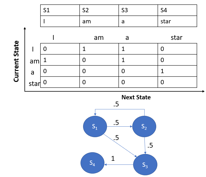
The above picture is an example of a transition graph where we have a closed-loop. Also, it bears a critical property of a Markov Chain: the probability of all edges leaving out of a specific node must be the sum of 1. See the S1 and S2 nodes. Also, observe that a Transient state is any state where the return probability is less than 1. See S1.
Let’s look at one more example.
Sentence 1: I had had too many chocolates.
Sentence 2: I had chocolates.
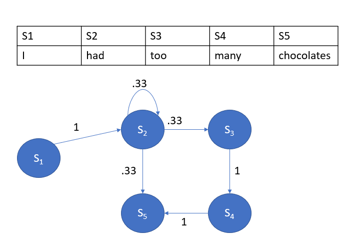
You can see a recurrence state over here with S2. There is some mathematical notation I want to explain here.
When we say a state j is accessible from state i, we write it as i→j, if pij(n)>0 for some n. We consider every state is accessible from itself since pii(0) =1. Also, Two states, i and j, are said to communicate, written as i↔j, in case they are reachable from each other. So, we can say, i↔j which, means i→j and j→i. In the Markov chain, Communication is an Equivalence relation. Meaning,
I. Every state communicates with itself, i↔i;(Reflexive)
II. Also, if i↔j, then j↔i;(Symmetric)
III. Also, if i↔j and j↔k, then i↔k. (Transitive)
Hence, the states of a Markov chain can be classified into communicating classes so that only members of the same class can communicate with each other. Two states i and j belong to the same class if and only if i↔j.
A Markov chain is Irreducible if all states communicate, meaning it belongs to one communication class. Also, in the case of two or more Communication classes, it’s known as the Reducible Markov chain.
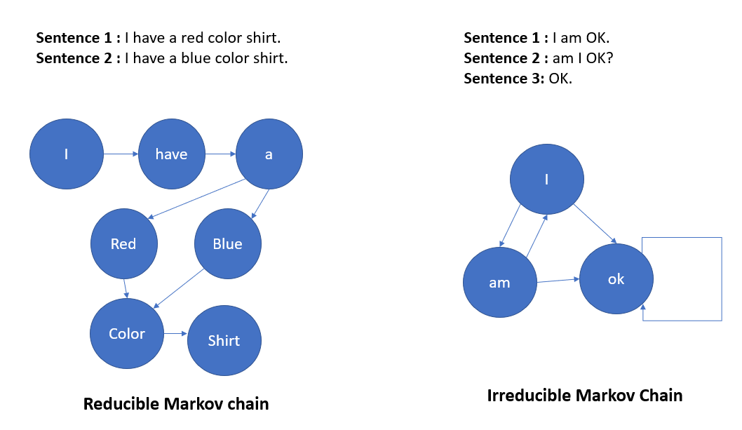
There is also a conception of Periodic and Aperiodic Markov state. I will give an example of both first. Let’s say we are going to measure the maximum temperature of consecutive days at a particular location. And below is the transition diagram.
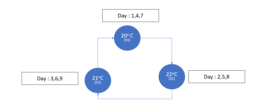
We can see that we only return to S1 at times n=3,6,⋯. So, p(n)00=0, if n is not divisible by 3. Such a state is called a periodic state with period d(0)=3. It can be shown that all states in the same communicating class are going to have the same period. A class is periodic if its states are periodic. Similarly, a class is aperiodic if its states are aperiodic. Also, a Markov chain is said to be aperiodic if all of its states are aperiodic. In other words, we can say a state S has a period K if K is GCD of the lengths of all the cycles that pass across S. If all the states in the Markov chain have a period K>1, it’s periodic else aperiodic. Another type of Markov chain is available, known as the Ergodic Markov chain. It is a combination of an irreducible and aperiodic chain.
I’ll give some intuition about Ergodic property as I feel in the present word being a data scientist you must have some notion of it. So, What is Ergodic property? The ergodic hypothesis says that the time spent by a system in some region of the phase space of microstates with the same energy is proportional to the volume of this region, i.e., that all accessible microstates are equally probable over a long period. The ergodic hypothesis says that the time spent by a system in some region of the phase space of microstates with the same energy is proportional to the volume of this region, i.e., that all accessible microstates are equally probable over a long period. Is it confusing, right? Let me simplify it a bit more. Ergodicity is a statement about how averages in one domain relate to another domain. It is about how we draw some conclusion about something while having information about something else. I hope the last statement can give you some correlation between the Markovian process and Ergodicity. Let me give you some examples now. You have been to a local football game. You are supporting your team. And there is a new player who is playing for the first time. During the match, he had scored a world-class solo goal while dribbling past five players. Now during the next game, you are confident he will score an important goal.
Another excellent example of this is In an election; each party gets some percentage of votes, party A receives x%, party B receives y%, and so on. However, it does not mean that throughout their lifetime, each person who has voted votes with party A in x% of elections, with B in y% of elections, and so on. I won’t give the mathematical explanation over here. You can do a little bit of research on it.
Basics of Transition Matrix
Now, let’s give some more intuitiveness about the Transition matrix. You have already become aware of the state transition diagram. Now it’s time for the Transition matrix. The basics of the Transition matrix are given below.
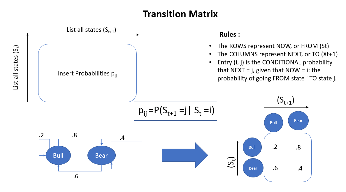
I will try to give some more examples, hope they will be sufficient to understand the concept. Let me share a very small sample. I hope the following diagram will be very much self-explanatory.
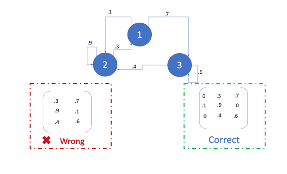
Now, let’s find out some properties of the transition matrix. Please try to correlate these properties with the above example.
Property 1: The value in the ith row and jth column marks the transition probabilities from state i to state j.
Property 2: Rows of this matrix must sum to 1, until and unless you do not have to go anywhere from the last state. In that case, the sum of that row will be 0.
Property 3: The transition matrix is square.
Property 4: The outcome of each state must be discrete.
Property 5: No state must remain constant with each generation.
For brevity, I will not use some more conceptual things as they may become a burden. Folks with advanced knowledge about linear algebra and probability can venture Hitting time, Hitting probability, Gamblers ruin problems. I have given some links for the same in reference.
Hidden Markov Model(HMM)
Before stating Hidden Markov Model, I’d like to clear intuition about posterior and prior probabilities. I know this is content-based on Bassian Statistics, but intuition will be helpful to understand the topic very well. Let’s begin. When do you see a word like ‘World,’ we consider it as a Noun. It is coming from our prior knowledge in the absence of data, or rather I’ll term it as context. So we see a word like ‘World,’ we put a higher probability with Noun than any other parts of speech. If we write ‘ World History,’ then ‘World’ becomes an Adjective in the context, right? Now you have data (context), and the probability of ‘World’ (Adjective) is higher than that of ‘World (Noun), given the data. This probability, wherein your condition on the data, is your posterior. Now the prior knowledge that I was talking about is hidden. We don’t know what factors motivated us to gain that kind of knowledge are. Now you may argue that you have studied English grammar well or read lots of English content for the preceding example. It is a specific case, but our base of prior ideas is generally always hidden while making any decision.
Let me give you another example. Suppose you are a fan of an English football club. You regularly follow their games in EPL. Even though they have a glorious history of performing at the top level in recent years, they are performance not up to the mark. On a Sunday, while watching a game of your favorite team with a bottom-listed club, your club is three goals down within 20 minutes of it. You are very upset. And suddenly, your doorbell rings. A neighbor walks in. He is looking for some old newspaper, which you need to search from a pile of a newspaper. As you were upset with your favorite team’s performance, you got cranky. You behaved very rudely and said you would do it later. Now your neighbor has seen you and talked with you some time. He used to think you were a very decent, respectful guy( prior belief). But the way you acted remains unclear to him. Maybe if he had been aware of the situation, he could have opted for a different time to visit. So here, what has driven your action to your neighbor, is hidden to him.
You can read the above example once again, and then please read what I am writing here. HMM requires an observable process Y(Our case, rude behavior of that person to his neighbor) whose outcomes are “influenced” by the consequences of X ( The lasting result of the football match) in a known way. Since X cannot be observed directly, the goal is to learn about X by watching Y.HMM has an additional requirement that the outcome of Y at time t=t0( particular moment of a time when the incident happened) may be “influenced” exclusively by the effect of X at t=t0 (At that time the result was against his favorite team )and that the outcomes of X and Y at t<t0 ( different time like maybe next morning) must not affect the outcome of Y at t=t0.
I hope now it’s a bit clear. Let me give you the mathematical definition of it. Let say Xn and Yn be a discrete-time stochastic process and n>=1. Then we can (Xn, Yn) is a hidden Markov model when
· Xn is a Markov process whose behavior is not visible(hidden).
· P(YnϵA|X1=x1,x2…….Xn=xn)=P(YnϵA|Xn=xn) for every n>=1.
For a continuous system, we also can define HMM. For more understanding, I am adding the common graphical interpretation that I have found in Wikipedia and trying to fit it into my example.
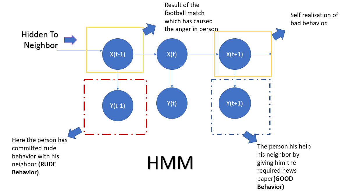
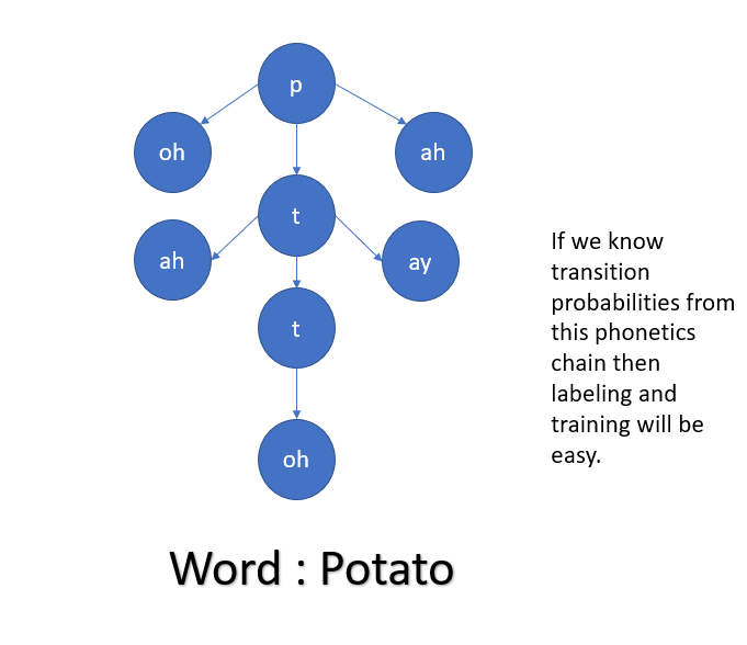
The usability of HMM in Speech processing is huge. Speech signals have different phonemes. Phonemes are segments of the spoken speech signal.A phoneme based HMM for say the word ‘cat’ would have /k/ /a/ and /t/ as states. In this approach, we will need to create an HMM for every word in the corpus and strengthen the model’s utterances. In the modern world, it’s more relevant as different people have different accent and phonetical property so using this model always helps to approximate the outcome statistically. Below is one example of the same.
Conclusion
The main weakness of the Markov chain is its incapability to represent non-transitive dependencies; As a result, many valuable independencies go unrepresented in the network. Bayesian networks use the richer language of directed graphs To overcome this deficiency, where the directions of the arrows permit us to distinguish actual dependencies from spurious dependencies induced by hypothetical observations. But still, the Markov chain has contributed hugely in the field of statistical analysis. In the current day, we say our world is a VUCA world. VUCA means Volatile, Uncertain, Complex, and Ambiguous. I feel the use of this kind of model can somewhat control the unpredictability of the VUCA world.
Markov Chain’s topic is so vast and complex that you can not cover it within a small time frame. Still, I am giving some references of some advanced issues once you get the notion of the Markov chain. Till then, Happy Learning.
Head on to our blog and read about the overview of the Markov Chain.
Reference of some advanced related topics and coding
Gamblers Ruin: http://www.statslab.cam.ac.uk/~rrw1/markov/M.pdf
Hitting time and hitting probability: https://gtribello.github.io/mathNET/HITTING_PROBABILITIES.html
Markov Random Field: Markov random fields (ermongroup.github.io)
Markov chain Monte Carlo: https://link.springer.com/article/10.3758/s13423-016-1015-8
Gibbs Sampling: Gibbs Sampling. Yet Another MCMC Method | by Cory Maklin | Towards Data Science
Bayesian Networks and Markov Random Fields: https://home.ttic.edu/~dmcallester/ttic10106/lectures/graphmodels/graphmodels.pdf
Coding Reference:
Check out: https://www.upgrad.com/blog/markov-chain-in-python-tutorial/
https://towardsdatascience.com/hidden-markov-model-implemented-from-scratch-72865bda430e
Note: To implement Markov Model, you must know the NUMPY library in Python very well.
YouTube Links:
I found the below links are very helpful while studying Markov Chain. You can look for it.
https://www.youtube.com/watch?v=cP3c2PJ4UHg
Used References:
[1] https://www.americanscientist.org/article/first-links-in-the-markov-chain
[2] https://jamesclear.com/domino-effect#:~:text=What%20is%20the%20Domino%20Effect,in%20related%20behaviors%20as%20well.&text=One%20habit%20led%20to%20another,patterns%20in%20your%20own%20life.
[3] https://www.stat.auckland.ac.nz/~fewster/325/notes/ch8.pdf
[4] https://thescipub.com/pdf/jmssp.2013.149.154.pdf
[5] https://www.quora.com/What-is-the-difference-between-a-recurrent-state-and-a-transient-state-in-a-Markov-Chain
[6] https://brilliant.org/wiki/absorbing-markov-chains/
[7] “Probabilistic reasoning in intelligent systems: Networks of Plausible Inference” written by Judea Pearl, chapter 3: Markov and Bayesian Networks: Two Graphical Representations of Probabilistic Knowledge, p.116:
[8] https://en.wikipedia.org/wiki/Hidden_Markov_model
[9] https://morioh.com/p/53d58990b989
[10] https://www.cs.cmu.edu/~avrim/598/chap5only.pdf
Reference for Exercise and Solutions: https://www.stat.berkeley.edu/~aldous/150/takis_exercises.pdf
Reference for some Thought-Provoking Research Paper and Patents using Markov Chain
https://arxiv.org/ftp/arxiv/papers/1601/1601.01304.pdf
https://pophealthmetrics.biomedcentral.com/articles/10.1186/s12963-020-00217-0
https://www.eajournals.org/wp-content/uploads/ON-THE-USE-OF-MARKOV-ANALYSIS-IN-MARKETING-OF.pdf
https://link.springer.com/article/10.1007/s42979-021-00768-5
https://patents.google.com/patent/CN101826114B/en
https://patents.justia.com/patent/9110817
The media shown in this article is not owned by Analytics Vidhya and are used at the Author’s discretion.


