This article was published as a part of the Data Science Blogathon
Introduction
In this article, we will learn very basic concepts of Recurrent Neural networks. So fasten your seatbelt, we are going to explore the very basic details of RNN with PyTorch.
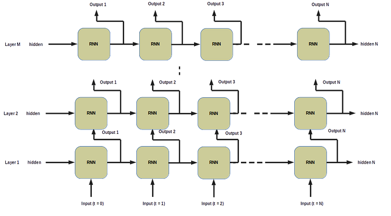
3 terminology for RNN:
- Input: Input to RNN
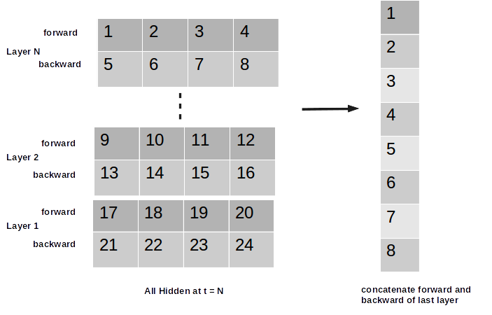
- Hidden: All hidden at last time step for all layers
- Output: All hidden at last layer for all time steps so that you can feed the hidden to next layer

Unidirectional RNN with PyTorch Image by Author
In the above figure we have N time steps (horizontally) and M layers vertically). We feed input at t = 0 and initially hidden to RNN cell and the output hidden then feed to the same RNN cell with next input sequence at t = 1 and we keep feeding the hidden output to the all input sequence. Implementation-wise in PyTorch, if you are new to PyTorch, I want to give you a very very useful tip, and this is really very important If you will follow I guarantee you will learn this quickly: And the tip is- Care more about the Shape
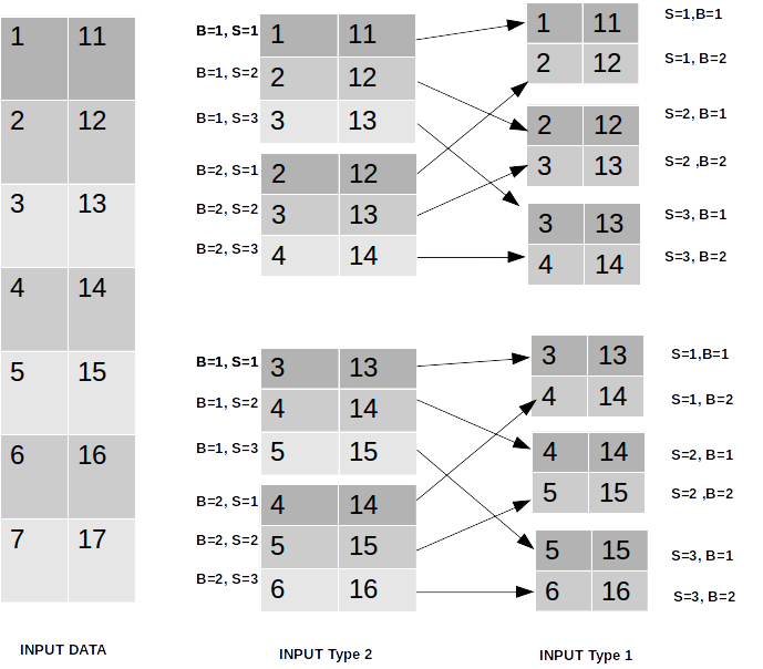
Assume we have the following one dimension array input data (row = 7 , columns=1 )
Data Type 1 (Image by author)
And we created sequential data and the label as shown above. Now we need to break this one into batches. Let’s say we take batch size = 2.

Input To RNN
Input data: RNN should have 3 dimensions. (Batch Size, Sequence Length and Input Dimension)
Sequence Length is the length of the sequence of input data (time step:0,1,2…N), the RNN learn the sequential pattern in the dataset. Here the grey colour part is sequence length so our sequence length = 3.
Suppose you have share market data on a daily basis (frequency = 1day) and you want that the network to learn the sequence of 30 days of data. So your sequence length will be 30.
Input Dimension or Input Size is the number of features or dimensions you are using in your data set. In this case, it is one (Columns/ Features). Suppose you have share market data with the following features: High, Low, Open and Close and you want to predict Close. In this case, you have input dimension = 4: High, Low, Open and Close. We will see the input dimension in more detail.
PyTorch takes input in two Shape :
Input Type 1: Sequence Length, Batch Size, Input Dimension
Input Type 2: Batch Size, Sequence Length, Input Dimension
If we choose Input type 1 our shape will be = 3, 2, 1
If we choose Input type 2 our shape will be = 2, 3, 1
Separate out the labels from input data because we only feed input sequences to the model, and then we will explore both of the Input shapes in detail. So we should move towards implementation. First I created a custom Dataset class that returns input sequences and labels. Here the input is a float array and seq_len is window size or the sequence length of input data.
class MyDaatset(Dataset):
    def __init__(self, input, seq_len):
        self.input = input
        self.seq_len = seq_len
    def __getitem__(self, item):
        return input[item:item + self.seq_len], input[item + self.seq_len]
    def __len__(self):
        return len(self.input) - self.seq_len
Define sequence from 1 to 7 and convert it to PyTorch tensor
input = np.arange(1,8).reshape(-1,1)
input = torch.tensor(input, dtype=torch.float)
Now we can call MyDataset class to get the data
ds = MyDaatset(input, 3)
As we have taken batch size = 2
dl = DataLoader(ds, batch_size=2)
for inp, label in dl:
    print(inp.numpy())
[[[1.]
  [2.]
  [3.]]
 [[2.]
  [3.]
  [4.]]]
[[[3.]
  [4.]
  [5.]]
 [[4.]
  [5.]
  [6.]]]
Now we have shapes as 2, 3, 1 (BS, SeqLen, Input Dim).
Suppose you have 2 input features for example feature 1 and feature 2

Then the input data will look like below. the only thing is the third dimension changed to 2 (2 is the number of features).
[[[1. 11.]
  [2. 12.]
  [3. 13.]]
 [[2. 12.]
  [3. 13.]
  [4. 14.]]]
[[[3. 13.]
  [4. 14.]
  [5. 15.]]
 [[4. 14.]
  [5. 15.]
  [6.16.]]]
Up to this point, we have discussed Input type 2: of shape (Batch Size, Sequence Length, Input Dimension). If we want to change this into Input type 1 we need to permute the input. To achieve this just switch batch dimension with sequence dimension in the input data, like below
inp.permute(1,0,2) # switch dimension 0 and dimension 1
[[[1. 11.]
  [2. 12.]]
 [[2. 12.]
  [3. 13.]]
 [[3. 13.]
  [4. 14.]]]
[[[3. 13.]
  [4. 14.]]
 [[4. 14.]
  [5. 15.]]
 [[5. 15.]
  [6.16.]]]
If you notice now the first dimension is 3, not 2, and it is our sequence length. And the second dimension is 2 which is batch size. And the third dimension is 2 which is the input dimension/ features. And our input shape is = (3, 2, 2) which is input type 1. If you are confusing a little bit then spend some time on this image-
Implementation
Let’s implement our small Recurrent Neural Net class, Inherit the base class nn.Module. HL_size = hidden size we can define as 32, 64, 128 (again better in 2’s power) and input size is a number of features in our data (input dimension). Here input size is 2 for data type 2 and 1 for data type 1.
batch_first=True means batch should be our first dimension (Input Type 2) otherwise if we do not define batch_first=True in RNN we need data in Input type 1 shape (Sequence Length, Batch Size, Input Dimension).
class RNNModel(torch.nn.Module):
    def __init__(self, input_size, HL_size):
        super(RNNModel, self).__init__()
        self.rnn = torch.nn.RNN(input_size=input_size,
                                hidden_size=Hidden Size(HS),
                                num_layers=number of stacked RNN,
                                bidirectional=True/False,
                                batch_first=True default is False)
        # If you want to use output for next layer then
        self.linear2 = torch.nn.Linear(#Direction * HS , Output_size)
        # If you want to use hidden for next layer then
        self.linear2 = torch.nn.Linear(HS , Output_size)
RNN returns output and is hidden.
Output
Output Shape: If we use batch_first=True, then output shape is (Batch Size, Seq Len, # Direction * Hidden Size). If we use batch_first=False, then output shape is ( Seq Len, Batch Size, No of Direction * Hidden Size)
Suppose if we consider data type 2 as input where seq_len is 3, batch is 2, hidden size = 128 and bidirectional = False then our output shape will be: (3, 2, 1 * 128) for batch_first=False and (2, 3, 1 * 128) for batch_first=True.
Hidden Shape: (No of Direction * num_layers, Batch Size, Hidden Size) which holds information about final hidden state. So most of the time we took hidden as an input in self.linear2.
Linear Transformation after RNN: If you are doing regression or binary classification then the output_size in Linear Transformation should be 1, If you are doing multi-class classification then Output_size will be a number of classes.
After __init__ you have to define forward class, this is the method of your RNN Class, which computes the hidden in the network. If you are using output (out in below code) as an input, then it means you will have hidden states for all time steps in the last layer, you need to select which time-step data you want to feed to the linear layer.
def forward(self, input):
    out, hidden_ = self.rnn(input)
    #out: Select which time step data you want for linear layer
    out = self.linear2(out)
If you want to use hidden_ as an input for the next layer just replace the last line with
out = self.linear2(hidden_)
In this case suppose If you have num_layer = 2, num_direction =2 then for each batch you will have 2 * 2= 4 hidden in the first dimension of hidden_, as hidden_ shape will be (4, BS, Hidden Size). Now you can select your input for the next layer from hidden_ (the way you want). For example, you can use both forward and backward direction of last hidden state from you hidden_ like below.

And we are done.
EndNotes
That is all about RNN in PyTorch. If not clear I advise you to do practice with code I am sure you will have a better understanding.


