


Introduction
With the advancement in deep learning, neural network architectures like recurrent neural networks (RNN and LSTM) and convolutional neural networks (CNN) have shown a decent improvement in performance in solving several Natural Language Processing (NLP) tasks like text classification, language modeling, machine translation, etc.
However, this performance of deep learning models in NLP pales in comparison to the performance of deep learning in Computer Vision.
One of the main reasons for this slow progress could be the lack of large labeled text datasets. Most of the labeled text datasets are not big enough to train deep neural networks because these networks have a huge number of parameters and training such networks on small datasets will cause overfitting.
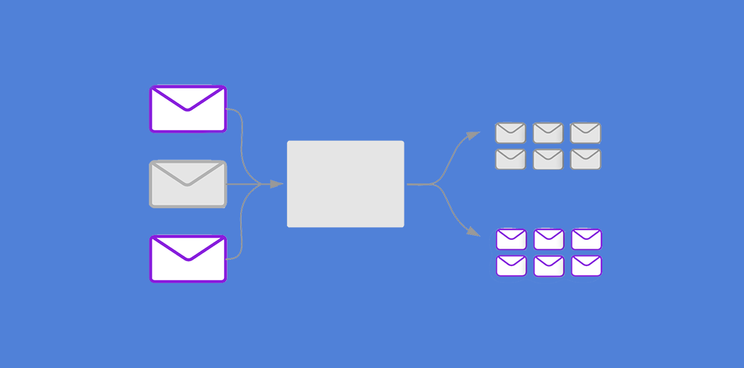
Another quite important reason for NLP lagging behind computer vision was the lack of transfer learning in NLP. Transfer learning has been instrumental in the success of deep learning in computer vision. This happened due to the availability of huge labeled datasets like Imagenet on which deep CNN based models were trained and later they were used as pre-trained models for a wide range of computer vision tasks.
That was not the case with NLP until 2018 when the transformer model was introduced by Google. Ever since the transfer learning in NLP is helping in solving many tasks with state of the art performance.
In this article, I explain how do we fine-tune BERT for text classification.
If you want to learn NLP from scratch, check out our course – Natural Language Processing (NLP) Using Python
Table of Contents
- Transfer Learning in NLP
- What is Model Fine-Tuning?
- Overview of BERT
- Fine-Tune BERT for Spam Classification
Transfer Learning in NLP
Transfer learning is a technique where a deep learning model trained on a large dataset is used to perform similar tasks on another dataset. We call such a deep learning model a pre-trained model. The most renowned examples of pre-trained models are the computer vision deep learning models trained on the ImageNet dataset. So, it is better to use a pre-trained model as a starting point to solve a problem rather than building a model from scratch.
This breakthrough of transfer learning in computer vision occurred in the year 2012-13. However, with recent advances in NLP, transfer learning has become a viable option in this NLP as well.
Most of the tasks in NLP such as text classification, language modeling, machine translation, etc. are sequence modeling tasks. The traditional machine learning models and neural networks cannot capture the sequential information present in the text. Therefore, people started using recurrent neural networks (RNN and LSTM) because these architectures can model sequential information present in the text.
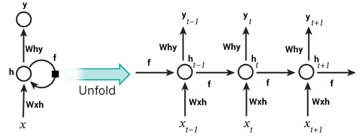
A typical RNN
However, these recurrent neural networks have their own set of problems. One major issue is that RNNs can not be parallelized because they take one input at a time. In the case of a text sequence, an RNN or LSTM would take one token at a time as input. So, it will pass through the sequence token by token. Hence, training such a model on a big dataset will take a lot of time.
So, the need for transfer learning in NLP was at an all-time high. In 2018, the transformer was introduced by Google in the paper “Attention is All You Need” which turned out to be a groundbreaking milestone in NLP.
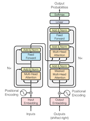
The Transformer – Model Architecture
(Source: https://arxiv.org/abs/1706.03762)
Soon a wide range of transformer-based models started coming up for different NLP tasks. There are multiple advantages of using transformer-based models, but the most important ones are:
-
First Benefit
These models do not process an input sequence token by token rather they take the entire sequence as input in one go which is a big improvement over RNN based models because now the model can be accelerated by the GPUs.
-
2nd Benefit
We don’t need labeled data to pre-train these models. It means that we have to just provide a huge amount of unlabeled text data to train a transformer-based model. We can use this trained model for other NLP tasks like text classification, named entity recognition, text generation, etc. This is how transfer learning works in NLP.
BERT and GPT-2 are the most popular transformer-based models and in this article, we will focus on BERT and learn how we can use a pre-trained BERT model to perform text classification.
What is Model Fine-Tuning?
BERT (Bidirectional Encoder Representations from Transformers) is a big neural network architecture, with a huge number of parameters, that can range from 100 million to over 300 million. So, training a BERT model from scratch on a small dataset would result in overfitting.
So, it is better to use a pre-trained BERT model that was trained on a huge dataset, as a starting point. We can then further train the model on our relatively smaller dataset and this process is known as model fine-tuning.
Different Fine-Tuning Techniques
- Train the entire architecture – We can further train the entire pre-trained model on our dataset and feed the output to a softmax layer. In this case, the error is back-propagated through the entire architecture and the pre-trained weights of the model are updated based on the new dataset.
- Train some layers while freezing others – Another way to use a pre-trained model is to train it partially. What we can do is keep the weights of initial layers of the model frozen while we retrain only the higher layers. We can try and test as to how many layers to be frozen and how many to be trained.
- Freeze the entire architecture – We can even freeze all the layers of the model and attach a few neural network layers of our own and train this new model. Note that the weights of only the attached layers will be updated during model training.
In this tutorial, we will use the third approach. We will freeze all the layers of BERT during fine-tuning and append a dense layer and a softmax layer to the architecture.
Overview of BERT
You’ve heard about BERT, you’ve read about how incredible it is, and how it’s potentially changing the NLP landscape. But what is BERT in the first place?
Here’s how the research team behind BERT describes the NLP framework:
“BERT stands for Bidirectional Encoder Representations from Transformers. It is designed to pre-train deep bidirectional representations from unlabeled text by jointly conditioning on both left and right context. As a result, the pre-trained BERT model can be fine-tuned with just one additional output layer to create state-of-the-art models for a wide range of NLP tasks.”
That sounds way too complex as a starting point. But it does summarize what BERT does pretty well so let’s break it down.
Firstly, BERT stands for Bidirectional Encoder Representations from Transformers. Each word here has a meaning to it and we will encounter that one by one in this article. For now, the key takeaway from this line is – BERT is based on the Transformer architecture. Secondly, BERT is pre-trained on a large corpus of unlabelled text including the entire Wikipedia (that’s 2,500 million words!) and Book Corpus (800 million words).
This pre-training step is half the magic behind BERT’s success. This is because as we train a model on a large text corpus, our model starts to pick up the deeper and intimate understandings of how the language works. This knowledge is the swiss army knife that is useful for almost any NLP task.
Third, BERT is a “deep bidirectional” model. Bidirectional means that BERT learns information from both the left and the right side of a token’s context during the training phase.
To learn more about the BERT architecture and its pre-training tasks, then you may like to read the below article:
Fine-Tune BERT for Spam Classification
Now we will fine-tune a BERT model to perform text classification with the help of the Transformers library. You should have a basic understanding of defining, training, and evaluating neural network models in PyTorch. If you want a quick refresher on PyTorch then you can go through the article below:
Link to Colab Notebook
Problem Statement
We have a collection of SMS messages. Some of these messages are spam and the rest are genuine. Our task is to build a system that would automatically detect whether a message is spam or not.
The dataset that we will be using for this use case can be downloaded from here (right-click and click on “Save link as…”).
I suggest you use Google Colab to perform this task so that you can use the GPU. Firstly, activate the GPU runtime on Colab by clicking on Runtime -> Change runtime type -> Select GPU.
Install Transformers Library
We will then install Huggingface’s transformers library. This library lets you import a wide range of transformer-based pre-trained models. Just execute the code below to install the library.
!pip install transformers
Import Libraries
Load Dataset
You would have to upload the downloaded spam dataset to your Colab runtime. Then read it into a pandas dataframe.
Output:
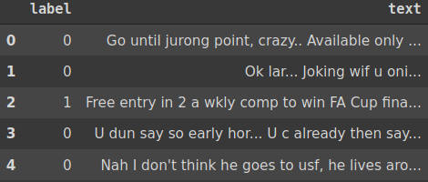
The dataset consists of two columns – “label” and “text”. The column “text” contains the message body and the “label” is a binary variable where 1 means spam and 0 means the message is not a spam.
Now we will split this dataset into three sets – train, validation, and test.
We will fine-tune the model using the train set and the validation set, and make predictions for the test set.
Import BERT Model and BERT Tokenizer
We will import the BERT-base model that has 110 million parameters. There is an even bigger BERT model called BERT-large that has 345 million parameters.
Python Code:
Let’s see how this BERT tokenizer works. We will try to encode a couple of sentences using the tokenizer.
Output:
{‘input_ids’: [[101, 2023, 2003, 1037, 14324, 2944, 14924, 4818, 102, 0],
[101, 2057, 2097, 2986, 1011, 8694, 1037, 14324, 2944, 102]],
‘attention_mask’: [[1, 1, 1, 1, 1, 1, 1, 1, 1, 0], [1, 1, 1, 1, 1, 1, 1, 1, 1, 1]]}
As you can see the output is a dictionary of two items.
- ‘input_ids’ contains the integer sequences of the input sentences. The integers 101 and 102 are special tokens. We add them to both the sequences, and 0 represents the padding token.
- ‘attention_mask’ contains 1’s and 0’s. It tells the model to pay attention to the tokens corresponding to the mask value of 1 and ignore the rest.
Tokenize the Sentences
Since the messages (text) in the dataset are of varying length, therefore we will use padding to make all the messages have the same length. We can use the maximum sequence length to pad the messages. However, we can also have a look at the distribution of the sequence lengths in the train set to find the right padding length.
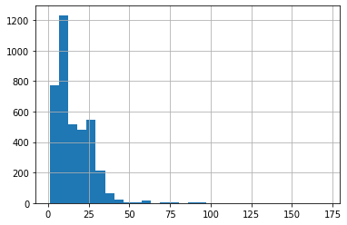
We can clearly see that most of the messages have a length of 25 words or less. Whereas the maximum length is 175. So, if we select 175 as the padding length then all the input sequences will have length 175 and most of the tokens in those sequences will be padding tokens which are not going to help the model learn anything useful and on top of that, it will make the training slower.
Therefore, we will set 25 as the padding length.
So, we have now converted the messages in train, validation, and test set to integer sequences of length 25 tokens each.
Next, we will convert the integer sequences to tensors.
Now we will create dataloaders for both train and validation set. These dataloaders will pass batches of train data and validation data as input to the model during the training phase.
Define Model Architecture
If you can recall, earlier I mentioned in this article that I would freeze all the layers of the model before fine-tuning it. So, let’s do it first.
This will prevent updating of model weights during fine-tuning. If you wish to fine-tune even the pre-trained weights of the BERT model then you should not execute the code above.
Moving on we will now let’s define our model architecture.
We will use AdamW as our optimizer. It is an improved version of the Adam optimizer. To learn more about it do check out this paper.
There is a class imbalance in our dataset. The majority of the observations are not spam. So, we will first compute class weights for the labels in the train set and then pass these weights to the loss function so that it takes care of the class imbalance.
Output: [0.57743559 3.72848948]
Fine-Tune BERT
So, till now we have defined the model architecture, we have specified the optimizer and the loss function, and our dataloaders are also ready. Now we have to define a couple of functions to train (fine-tune) and evaluate the model, respectively.
We will use the following function to evaluate the model. It will use the validation set data.
Now we will finally start fine-tuning of the model.
Output:
Training Loss: 0.592
Validation Loss: 0.567

Epoch 5 / 10
Batch 50 of 122.
Batch 100 of 122.

Evaluating...

Training Loss: 0.566
Validation Loss: 0.543

Epoch 6 / 10
Batch 50 of 122.
Batch 100 of 122.

Evaluating...

Training Loss: 0.552
Validation Loss: 0.525

Epoch 7 / 10
Batch 50 of 122.
Batch 100 of 122.

Evaluating...

Training Loss: 0.525
Validation Loss: 0.498

Epoch 8 / 10
Batch 50 of 122.
Batch 100 of 122.

Evaluating...

Training Loss: 0.507
Validation Loss: 0.477

Epoch 9 / 10
Batch 50 of 122.
Batch 100 of 122.

Evaluating...

Training Loss: 0.488
Validation Loss: 0.461

Epoch 10 / 10
Batch 50 of 122.
Batch 100 of 122.

Evaluating...

Training Loss: 0.474
Validation Loss: 0.454
You can see that the validation loss is still decreasing at the end of the 10th epoch. So, you may try a higher number of epochs. Now let’s see how well it performs on the test dataset.
Make Predictions
To make predictions, we will first of all load the best model weights which were saved during the training process.
Once the weights are loaded, we can use the fine-tuned model to make predictions on the test set.
Let’s check out the model’s performance.
Output:
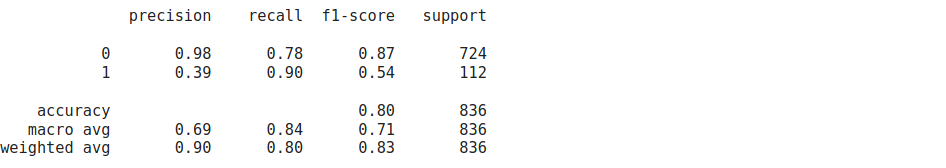
Both recall and precision for class 1 are quite high which means that the model predicts this class pretty well. However, our objective was to detect spam messages, so misclassifying class 1 (spam) samples is a bigger concern than misclassifying class 0 samples. If you look at the recall for class 1, it is 0.90 which means that the model was able to correctly classify 90% of the spam messages. However, precision is a bit on the lower side for class 1. It means that the model misclassifies some of the class 0 messages (not spam) as spam.
Link to Colab Notebook
End Notes
To summarize, in this article, we fine-tuned a pre-trained BERT model to perform text classification on a very small dataset. I urge you to fine-tune BERT on a different dataset and see how it performs. You can even perform multiclass or multi-label classification with the help of BERT. In addition to that, you can even train the entire BERT architecture as well if you have a bigger dataset.
In case you are looking for a roadmap to becoming an expert in NLP read the following article-
You may use the comment section in case you have any thoughts to share or have any doubts.