This article was published as a part of the Data Science Blogathon.
Introduction
Sentiment Analysis is an NLP application that identifies a text corpus’s emotional or sentimental tone or opinion. Usually, emotions or attitudes towards a topic can be positive, negative, or neutral. This makes sentiment analysis a text classification task. Examples of positive, negative, and neutral expressions are:
“I enjoyed the movie!” – Positive
“I am not sure if I liked the movie.” – Neutral
“It was the most terrible movie I have ever seen.” – Negative
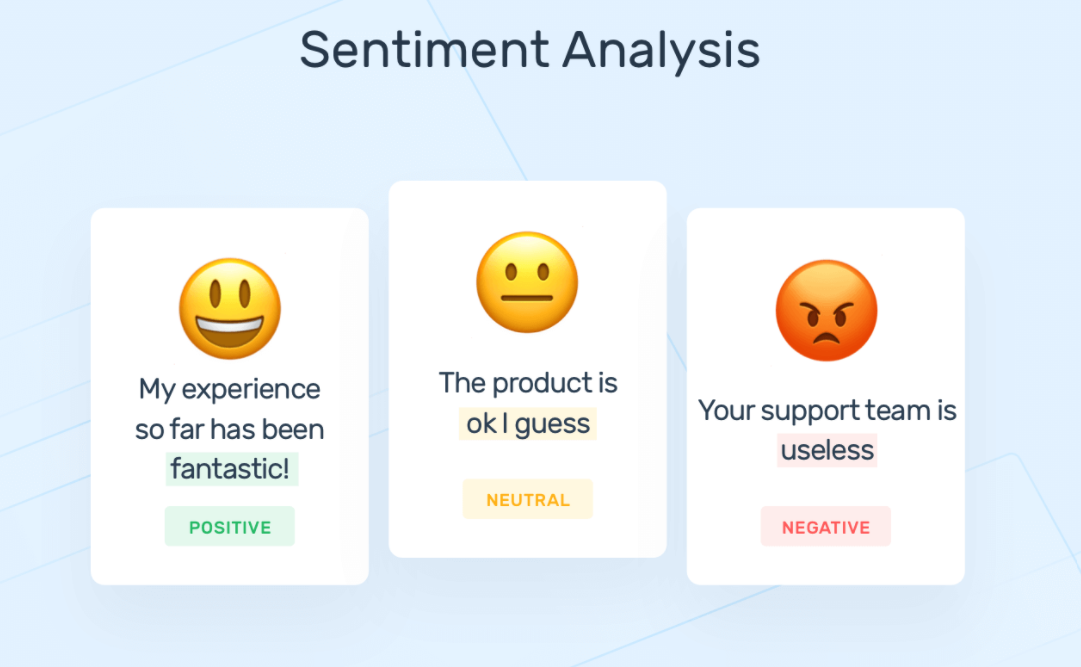
Sentiment analysis is a potent tool with varied applications across industries. It is helpful for social media and brand monitoring, customer support and feedback analysis, market research, etc. A new product’s target audience or demographics can be identified by performing sentiment analysis on initial customer feedback received, and it can help evaluate the success of a marketing campaign. As sentiment analysis grows more and more useful in the industry, it becomes essential for us to learn how to perform it. This article will know how to do sentiment analysis on movie reviews using LSTMs.
What is LSTM?
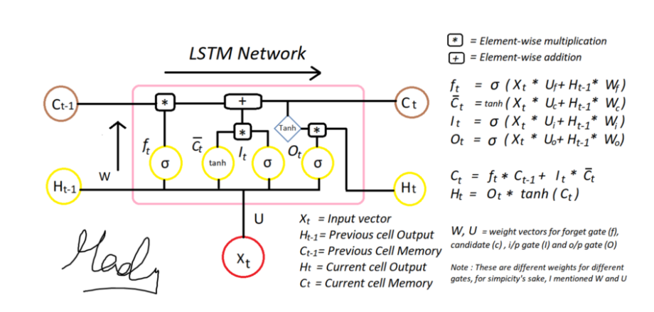
Recurrent neural networks (RNNs) are a form of Artificial Neural networks that can memorize arbitrary-length sequences of input patterns by capturing connections between sequential data types. However, due to stochastic gradients’ failure, RNNs are unable to detect long-term dependencies in lengthy sequences. Several novel RNN models, notably LSTM, were proposed to address this issue. LSTM networks are RNN extensions designed to learn sequential (temporal) data and their long-term connections more precisely than standard RNNs. They are commonly used in deep learning applications such as stock forecasting, speech recognition, natural language processing, etc.
Loading the Dataset
We will be performing sentiment analysis on 50k IMDB movie reviews, and the dataset is balanced with 25k positive and 25k negative movie reviews. You can download the dataset from here. We start with importing necessary packages for text manipulation and model building.
import re
import pandas as pd
import numpy as np
from sklearn.preprocessing import LabelEncoder
from sklearn.model_selection import train_test_split
from keras.preprocessing.text import Tokenizer
from keras.preprocessing.sequence import pad_sequences
import keras
from sklearn.metrics import classification_report
from sklearn.metrics import accuracy_score
import math
import nltk
We load the dataset into a pandas dataframe with the help of the following code :
data = pd.read_csv('IMDB Dataset.csv')
data
The data looks like this :
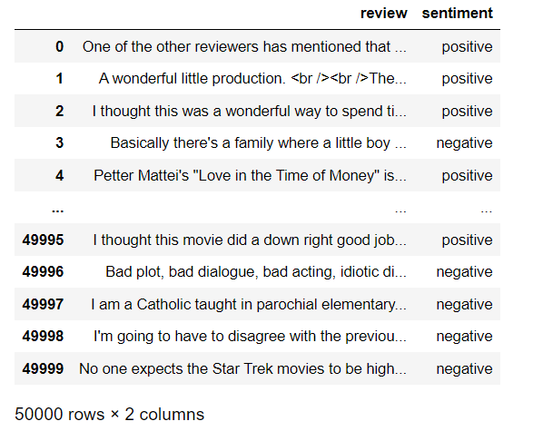
Source: Screenshot from my Jupyter Notebook
Data Preprocessing
First, we need to remove HTML tags, URLs, and non-alphanumeric characters from the reviews. We do that with the help of the remove_tags function, and Regex functions are used for easy string manipulation.
def remove_tags(string):
    removelist = ""
    result = re.sub('','',string)          #remove HTML tags
    result = re.sub('https://.*','',result)   #remove URLs
    result = re.sub(r'[^w'+removelist+']', ' ',result)    #remove non-alphanumeric characters
    result = result.lower()
    return result
data['review']=data['review'].apply(lambda cw : remove_tags(cw))
We also need to remove stopwords from the corpus. Stopwords are commonly used words like ‘and’, ‘the’, ‘at’ that do not add any special meaning or significance to a sentence. A list of stopwords are available with nltk, and they can be removed from the corpus using the following code :
nltk.download('stopwords')
from nltk.corpus import stopwords
stop_words = set(stopwords.words('english'))
data['review'] = data['review'].apply(lambda x: ' '.join([word for word in x.split() if word not in (stop_words)]))
We now perform lemmatization on the text. Lemmatization is a useful technique in NLP to obtain the root form of words, known as lemmas. For example, the lemma of the words reading, reads, read is read. This helps save unnecessary computational overhead in trying to decipher entire words, as the meanings of most words are well-expressed by their separate lemmas. We perform lemmatization using the WordNetLemmatizer() from nltk. The text is first broken into individual words using the WhitespaceTokenizer() from nltk. We write a function lemmatize_text to perform lemmatization on the individual tokens.
w_tokenizer = nltk.tokenize.WhitespaceTokenizer()
lemmatizer = nltk.stem.WordNetLemmatizer()
def lemmatize_text(text):
    st = ""
    for w in w_tokenizer.tokenize(text):
        st = st + lemmatizer.lemmatize(w) + " "
    return st
data['review'] = data.review.apply(lemmatize_text)
data
The processed data looks like this :
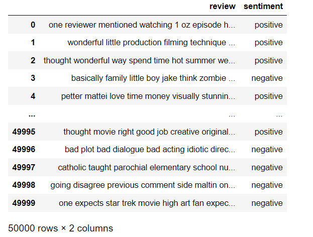
Next, we print some basic statistics about the dataset and check if the dataset is balanced or not (equal number of all labels). Ideally, the dataset should be balanced because a severely imbalanced dataset can be challenging to model and require specialized techniques.
s = 0.0
for i in data['review']:
    word_list = i.split()
    s = s + len(word_list)
print("Average length of each review : ",s/data.shape[0])
pos = 0
for i in range(data.shape[0]):
    if data.iloc[i]['sentiment'] == 'positive':
        pos = pos + 1
neg = data.shape[0]-pos
print("Percentage of reviews with positive sentiment is "+str(pos/data.shape[0]*100)+"%")
print("Percentage of reviews with negative sentiment is "+str(neg/data.shape[0]*100)+"%")
>>Average length of each review :  119.57112
>>Percentage of reviews with positive sentiment is 50.0%
>>Percentage of reviews with negative sentiment is 50.0%
Encoding Labels and Making Train-Test Splits
We use the LabelEncoder() from sklearn.preprocessing to convert the labels (‘positive’, ‘negative’) into 1’s and 0’s respectively.
reviews = data['review'].values
labels = data['sentiment'].values
encoder = LabelEncoder()
encoded_labels = encoder.fit_transform(labels)
Finally, we split the dataset into train and test parts using train_test_split from sklearn.model_selection. We use 80% of the dataset for training and 20% for testing.
train_sentences, test_sentences, train_labels, test_labels = train_test_split(reviews, encoded_labels, stratify = encoded_labels)
Before being fed into the LSTM model, the data needs to be padded and tokenized:
- Tokenizing: Keras’ inbuilt tokenizer API has fit the dataset, which splits the sentences into words and creates a dictionary of all unique words found and their uniquely assigned integers. Each sentence is converted into an array of integers representing all the individual words present in it.
- Sequence Padding: The array representing each sentence in the dataset is filled with zeroes to the left to make the size of the array ten and bring all collections to the same length.
# Hyperparameters of the model
vocab_size = 3000 # choose based on statistics
oov_tok = ''
embedding_dim = 100
max_length = 200 # choose based on statistics, for example 150 to 200
padding_type='post'
trunc_type='post'
# tokenize sentences
tokenizer = Tokenizer(num_words = vocab_size, oov_token=oov_tok)
tokenizer.fit_on_texts(train_sentences)
word_index = tokenizer.word_index
# convert train dataset to sequence and pad sequences
train_sequences = tokenizer.texts_to_sequences(train_sentences)
train_padded = pad_sequences(train_sequences, padding='post', maxlen=max_length)
# convert Test dataset to sequence and pad sequences
test_sequences = tokenizer.texts_to_sequences(test_sentences)
test_padded = pad_sequences(test_sequences, padding='post', maxlen=max_length)
Building the Model
A Keras sequential model is built. It is a linear stack of the following layers :
- An embedding layer of dimension 100 converts each word in the sentence into a fixed-length dense vector of size 100. The input dimension is set as the vocabulary size, and the output dimension is 100. Each word in the input will hence get represented by a vector of size 100.
- A bidirectional LSTM layer of 64 units.
- A dense (fully connected) layer of 24 units with relu activation.
- A dense layer of 1 unit and sigmoid activation outputs the probability of the review is positive, i.e. if the label is 1.
The code for building the model :
# model initialization
model = keras.Sequential([
    keras.layers.Embedding(vocab_size, embedding_dim, input_length=max_length),
    keras.layers.Bidirectional(keras.layers.LSTM(64)),
    keras.layers.Dense(24, activation='relu'),
    keras.layers.Dense(1, activation='sigmoid')
])
# compile model
model.compile(loss='binary_crossentropy',
              optimizer='adam',
              metrics=['accuracy'])
# model summary
model.summary()
The model is compiled with binary cross-entropy loss and adam optimizer. Since we have a binary classification problem, binary cross-entropy loss is used. The Adam optimizer uses stochastic gradient descent to train deep learning models, and it compares each of the predicted probabilities to the actual class label (0 or 1). Accuracy is used as the primary performance metric. The model summary can be seen below :
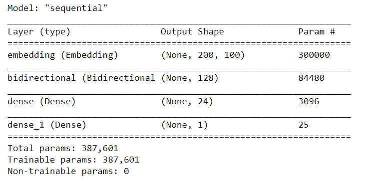
Source: Screenshot from my Jupyter Notebook
Model Training and Evaluation
The model is trained for five epochs.
num_epochs = 5
history = model.fit(train_padded, train_labels,
                    epochs=num_epochs, verbose=1,
                    validation_split=0.1)
The model is evaluated by calculating its accuracy. Accuracy of classification is calculated by dividing the number of correct predictions by the total number of predictions.
prediction = model.predict(test_padded)
# Get labels based on probability 1 if p>= 0.5 else 0
pred_labels = []
for i in prediction:
    if i >= 0.5:
        pred_labels.append(1)
    else:
        pred_labels.append(0)
print("Accuracy of prediction on test set : ", accuracy_score(test_labels,pred_labels))
The accuracy of prediction on the test set comes out to be 87.27%! You can improve the accuracy further by playing around with the model hyperparameters, further tuning the model architecture or changing the train-test split ratio. You should also train the model for a more significant number of epochs, and we stopped at five epochs because of the computational time. Ideally, it would help prepare the model until the train and test losses converge.
Using the model to determine the sentiment of unseen movie reviews
We can use our trained model to determine the sentiment of new unseen movie reviews not present in the dataset. Each new text must be tokenized and padded before being fed as input to the model. The model.predict() function returns the probability of the positive review. If the probability is more significant than 0.5, we consider the study to be positive, else negative.
# reviews on which we need to predict
sentence = ["The movie was very touching and heart whelming",
            "I have never seen a terrible movie like this",
            "the movie plot is terrible but it had good acting"]
# convert to a sequence
sequences = tokenizer.texts_to_sequences(sentence)
# pad the sequence
padded = pad_sequences(sequences, padding='post', maxlen=max_length)
# Get labels based on probability 1 if p>= 0.5 else 0
prediction = model.predict(padded)
pred_labels = []
for i in prediction:
    if i >= 0.5:
        pred_labels.append(1)
    else:
        pred_labels.append(0)
for i in range(len(sentence)):
    print(sentence[i])
    if pred_labels[i] == 1:
        s = 'Positive'
    else:
        s = 'Negative'
    print("Predicted sentiment : ",s)
The output looks very promising!

Source: Screenshot from my Jupyter Notebook
Conclusion
Sentiment analysis, like any other classification task, can be performed with many different machine learning and deep learning models, such as Naive Bayes, KNN, SVM or CNN, ANN, etc. Now that you know its basics go ahead and explore other models to perform sentiment analysis.
Thank you for reading.
You can read here about how to use CNNs for text classification!
Feel free to connect with me over email: [email protected]
The media shown in this article is not owned by Analytics Vidhya and are used at the Author’s discretion.


