Introduction
Agriculture is the main source of food in India. During the crop cycle, many plant diseases can occur and can affect the crop. Identification and classification of plant disease at the leaf level is a crucial part of crop management and is important in the early detection and diagnosis of plant diseases. Traditionally, the classification of plant diseases has been performed by farmers using manual methods like manual inspection or field observations. However, this process is time-consuming and error-prone, which is why there is a need for an intelligent system that can automatically classify images based on plant leaf diseases.
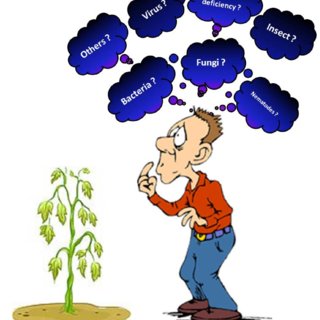
This article will solve this problem using data science and deep learning. We will use Python, and a CNN named AlexNet for this project. In this article, you will learn the architecture of AlexNet, the workflow of building a deep learning model, and how to build a ready-to-use classification model for plant diseases.
Table of Contents
Here is a brief overview of the contents of this article:
- Introduction
- Problem Statement
- Proposed Solution
- Description of the dataset
- Getting started with AlexNet
- ReLu activation in AlexNet
- Local Response Normalization in AlexNet
- Issues with AlexNet
- Methodology
- Code implementation
- Conclusion
Problem Statement
We will address the following problem statement: “Identify the illness that a plant leaf contains, given an image showing the disease.”
That is, we need to tell the farmer the name of the illness the leaf is infected with when we get a random plant leaf photograph from them showing a crop disease.
Proposed Solution
The proposed solution to this problem is to develop a deep learning model capable of identifying and classifying plant leaf images based on the disease they possess. We will use AlexNet, an eight-layered convolution network, in this project.
Description of the Dataset
For this project, we will use the PlantVillage dataset available on Kaggle.
The PlantVillage dataset, a leaf disease image dataset, has been taken from Kaggle. The dataset consists of test and training images for 38 classes: bacterial spot, black mold, grey mold, late blight, powdery mildew, and healthy leaves in apples, potato, tomato, corn, cherry, and soy crops. There are 70295 images in total, each with 227 * 227 pixels.
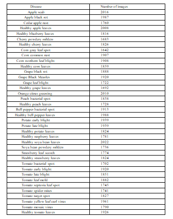
Several images of the leaf diseases are available in the dataset that has been used.
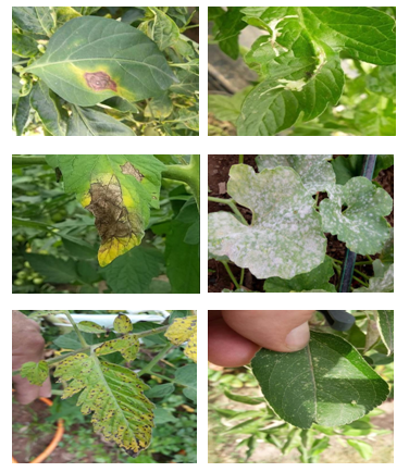
A few sample images from the dataset are shown below:
Getting Started with AlexNet
A CNN architecture named AlexNet was chosen as the 2012 LSVRC competition winner. Research teams compete to attain higher accuracy on various visual recognition tasks in the Large Scale Visual Recognition Challenge by evaluating their algorithms on a sizable dataset of annotated images (ImageNet). There are over 1.2 million training images, 50,000 validation images, and 150,000 testing images. By removing the central 256×256 patch from each image, the model builders imposed a fixed size of 256×256 pixels.
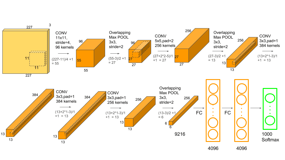
AlexNet’s architecture consists of 8 convolutional layers, of which 5 convolutional layers and three ANN layers. Each of the convolution layers is followed by a max pooling layer. Its architecture is easy to understand. It uses ReLu activation and involves overlapping max pooling. The following image shows the architecture of AlexNet.
Features of AlexNet:
- Kernels in the 2nd, 4th, and 5th convolution layers are interlinked to those kernels in the previous layers that lie on the same GPU.
- The neurons present in the fully connected layers are interconnected with each other.
- ReLu activation is applied to the output of every convolution layer and in the simple artificial neural network structure.
ReLu Activation in AlexNet
Usually, the sigmoid or tanh function is used as an activation function in deep learning networks. However, AlexNet employs a non-linear activation function called Rectified Linear Unit activation. The former activation functions saturate quickly, and training on GPUs using these functions is not easy, so non-linearity in ReLu helps with effective learning. The following equation gives the working functionality in ReLu:
𝑓(𝑥) = 𝑚𝑎𝑥(0, 𝑥)
The derivative of the above equation is 1 if x > 0 and 0 in other cases. Unlike sigmoid and tanh, which have the specific boundary of derivative values, the ReLu function has only two values for its derivative.
The vanishing gradient descent problem present when using sigmoid and tanh functions is not experienced during ReLu activation.
Local Response Normalization in AlexNet
Normalization is a crucial part of neural networks that use nonlinear activation functions. Nonlinear activation functions do not have a bounded set of outputs like linear ones, so we use normalization to restrict the unbounded activation outputs. Local response normalization helps the generalization process. ReLU was chosen as the activation function instead of the then-common tanh and sigmoid, which led to the usage of “local response normalization” (LRN) in the AlexNet architecture.
In addition to the aforementioned justification, the use of LRN was made to promote lateral inhibition. A neuron’s ability to lessen its neighbors’ action is a notion in neuroscience. This lateral inhibition function in DNNs is employed to perform local contrast enhancement such that the highest pixel values are used as local stimulation for the following layers. The pixel values of a feature map of a nearby neighborhood are square-normalized using LRN, a non-trainable layer.
Issues with AlexNet
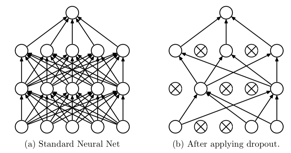
Since the original architecture of AlexNet was developed using large amounts of data, overfitting is a problem when using this CNN. Data augmentation and dropout techniques were used to overcome this problem. By using dropout layers, the performance of the CNN architecture was seen to improve. The dropped attributes do not participate in forward and backward propagation, which reduces the complex co-adaptations of neurons. This allows the network to learn more robust features. Dropout is used in the first two layers in the fully connected structure of AlexNet.
Methodology
The steps involved in this project are as follows:
- Import Libraries
- Define batch specifications
- Load the dataset
- Building the AlexNet architecture
- Compile the model
- Training and validation
- Saving the model
- Testing the model with a test image
Code Implementation
Now that we have written down the project’s steps. Let us start the practical implementation.
Step 1. Import Libraries
The first step in a machine learning or data science project would be to import the necessary libraries.
import numpy as np
import pandas as pd
import matplotlib.pyplot as plt
import tensorflow as tf
from tensorflow.keras import layers
from time import perf_counter
import os
import seaborn as sns
from PIL import Image
from PIL import ImageEnhance
from skimage.io import imread
import matplotlib.pyplot as plt
import os, random, pathlib, warnings, itertools, math
warnings.filterwarnings("ignore")
import tensorflow as tf
import tensorflow.keras.backend as K
from sklearn.metrics import confusion_matrix
from tensorflow.keras import models
from tensorflow.keras.models import Model
from tensorflow.keras.models import load_model
from tensorflow.keras.preprocessing import image
from keras.preprocessing.image import load_img,img_to_array
from tensorflow.keras.layers import Dense, Dropout, Flatten, Input, LeakyReLU
from tensorflow.keras.layers import BatchNormalization, Activation, Conv2D
from tensorflow.keras.applications import ResNet101V2
from tensorflow.keras.models import Sequential
from tensorflow.keras.preprocessing.image import ImageDataGenerator
from tensorflow.keras.layers import Dense, Flatten, MaxPooling2D, Dense, Dropout
K.clear_session()
For building the AlexNet model, we are going to need the TensorFlow and Keras libraries. While Numpy, Pandas, and Scikit Learn are other purposes.
Step 2: Define Batch Specifications
Next, let us define the batch specifications. Here, batch size refers to the number of training images we will use in one loop. The image’s height and width are specified to ensure that all images are of uniform size.
## Defining batch specfications
batch_size = 100
img_height = 250
img_width = 250
Step 3: Load the Dataset
If you glance at the dataset, you will see different folders available for training and validation. Hence, we shall load them separately.
3.1 Load the training data
training_data = tf.keras.preprocessing.image_dataset_from_directory("/kaggle/input/new-plant-diseases-dataset/New Plant Diseases Dataset(Augmented)/New Plant Diseases Dataset(Augmented)/train",
    seed=42,
    image_size= (img_height, img_width),
    batch_size=batch_size
)
Then, the validation data is imported in the same way using the same parameters.
3.2 Getting the Validation Data
validation_data = tf.keras.preprocessing.image_dataset_from_directory("/kaggle/input/new-plant-diseases-dataset/New Plant Diseases Dataset(Augmented)/New Plant Diseases Dataset(Augmented)/valid",
    seed=42,
    image_size= (img_height, img_width),
    batch_size=batch_size
)

3.3 Storing the Label Names
The dataset consists of images of 38 different plant leaf diseases. It would be easier for us to get to know the class labels, the disease names, to use them in the later steps.
target_names = training_data.class_names
print(target_names)
Output:

Step 4. Building AlexNet Architecture
Moving ahead, the next step is to build the model for classifying the plant leaf images. As already mentioned, we are going to use the AlexNet CNN architecture. The code for this is shown below.
model = Sequential()
# 1st Convolutional Layer
model.add(Conv2D(filters = 96, input_shape = (250, 250, 3),
kernel_size = (11, 11), strides = (4, 4),
padding = 'valid'))
model.add(Activation('relu'))
# Max-Pooling
model.add(MaxPooling2D(pool_size = (2, 2),
strides = (2, 2), padding = 'valid'))
# Batch Normalisation
model.add(BatchNormalization())
# 2nd Convolutional Layer
model.add(Conv2D(filters = 256, kernel_size = (11, 11),
strides = (1, 1), padding = 'valid'))
model.add(Activation('relu'))
# Max-Pooling
model.add(MaxPooling2D(pool_size = (2, 2), strides = (2, 2),
padding = 'valid'))
# Batch Normalisation
model.add(BatchNormalization())
# 3rd Convolutional Layer
model.add(Conv2D(filters = 384, kernel_size = (3, 3),
strides = (1, 1), padding = 'valid'))
model.add(Activation('relu'))
# Batch Normalisation
model.add(BatchNormalization())
# 4th Convolutional Layer
model.add(Conv2D(filters = 384, kernel_size = (3, 3),
strides = (1, 1), padding = 'valid'))
model.add(Activation('relu'))
# Batch Normalisation
model.add(BatchNormalization())
# 5th Convolutional Layer
model.add(Conv2D(filters = 256, kernel_size = (3, 3),
strides = (1, 1), padding = 'valid'))
model.add(Activation('relu'))
# Max-Pooling
model.add(MaxPooling2D(pool_size = (2, 2), strides = (2, 2),
padding = 'valid'))
# Batch Normalisation
model.add(BatchNormalization())
# Flattening
model.add(Flatten())
# 1st Dense Layer
model.add(Dense(4096, input_shape = (250*250*3, )))
model.add(Activation('relu'))
# Add Dropout to prevent overfitting
model.add(Dropout(0.4))
# Batch Normalisation
model.add(BatchNormalization())
# 2nd Dense Layer
model.add(Dense(4096))
model.add(Activation('relu'))
# Add Dropout
model.add(Dropout(0.4))
# Batch Normalisation
model.add(BatchNormalization())
# Output Softmax Layer
model.add(Dense(len(target_names)))
model.add(Activation('softmax'))
model.summary()
Output:
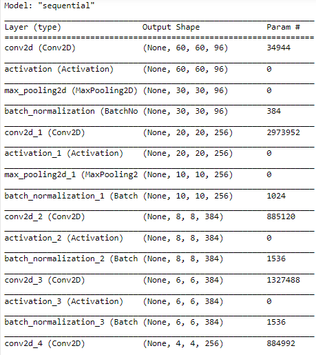
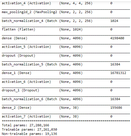
This is a summary of the AlexNet model that has been built. It contains 5 convolution layers, 3 max-pooling layers and 2 dropout layers towards the end.
Step 5. Compile the Model
Next, we compile the model by defining the evaluation metrics and losses to be considered.
model.compile(optimizer='adam',loss='sparse_categorical_crossentropy', metrics=['accuracy'])
Step 6. Training and Validation
Once the AlexNet model is compiled, we train it using the training dataset and validate it. We will use 10 epochs and see the model’s accuracy over the validation data.
my_model = model.fit(training_data,validation_data= validation_data,epochs = 10)
Output:
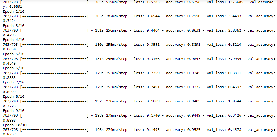
It can be seen that the model has a validation accuracy of 87%.
Step 7. Saving the Model
model.save("/kaggle/working/AlexNetModel.hdf5")
model.save("AlexNetModel.hdf5")
Next up, we save the model from being used for deployment.
Step 8. Testing the Model with a Test Image
Finally, we test the saved model on a sample image.
import imageio
import tensorflow
from tensorflow import keras
import numpy as np
from tensorflow.keras.preprocessing.image import img_to_array, load_img
from tensorflow.keras.models import load_model
from PIL import Image
target_names = ['Apple___Apple_scab', 'Apple___Black_rot', 'Apple___Cedar_apple_rust', 'Apple___healthy', 'Blueberry___healthy', 'Cherry_(including_sour)___Powdery_mildew', 'Cherry_(including_sour)___healthy', 'Corn_(maize)___Cercospora_leaf_spot Gray_leaf_spot', 'Corn_(maize)___Common_rust_', 'Corn_(maize)___Northern_Leaf_Blight', 'Corn_(maize)___healthy', 'Grape___Black_rot', 'Grape___Esca_(Black_Measles)', 'Grape___Leaf_blight_(Isariopsis_Leaf_Spot)', 'Grape___healthy', 'Orange___Haunglongbing_(Citrus_greening)', 'Peach___Bacterial_spot', 'Peach___healthy', 'Pepper,_bell___Bacterial_spot', 'Pepper,_bell___healthy', 'Potato___Early_blight', 'Potato___Late_blight', 'Potato___healthy', 'Raspberry___healthy', 'Soybean___healthy', 'Squash___Powdery_mildew', 'Strawberry___Leaf_scorch', 'Strawberry___healthy', 'Tomato___Bacterial_spot', 'Tomato___Early_blight', 'Tomato___Late_blight', 'Tomato___Leaf_Mold', 'Tomato___Septoria_leaf_spot', 'Tomato___Spider_mites Two-spotted_spider_mite', 'Tomato___Target_Spot', 'Tomato___Tomato_Yellow_Leaf_Curl_Virus', 'Tomato___Tomato_mosaic_virus', 'Tomato___healthy']
def run(source = None):
    model = tensorflow.keras.models.load_model('C:/Users/HP/OneDrive/Desktop/AlexNet/alexnet_model/AlexNetModel.hdf5')
    img = imageio.imread(source)
    img = Image.fromarray(img).resize((224, 224))
    x = img_to_array(img)
    x = np.expand_dims(img, axis=0)
    x = x/255
    prediction = model.predict(x)
    print("Predicted Image is:",target_names[np.argmax(prediction)])
run(source=r'C:UsersHPOneDriveDesktopAlexNettestTomatoYellowCurlVirus4.JPG')
Here in the run command, you can give the path location of your test image and get the output. The above code can be used for further deploying the model.
Conclusion
This brings the classification of plant disease to a close. Reviewing our work on this project will be helpful. We started by defining the problem statement and learning about Alexnet’s operation, design, ReLu activation, and problems encountered while using it. Next, we looked at the process of implementing the project using Python and deep learning. Finally, we got into implementing our learnings through a practical code implementation.
The key takeaways from this article are:
- Plant diseases may seriously threaten crops. Therefore, it is critical to identify them early so you can take the necessary precautions.
- One of the modern ways of diagnosing plant diseases is to classify images using an automated system depending on the illness.
- AlexNet provides pretty good image categorization accuracy.
I hope you like my article on “Plant Disease Classification Using AlexNet.” You can connect with me here on LinkedIn.
The media shown in this article are not owned by Analytics Vidhya and are used at the author’s discretion.


