This article was published as a part of the Data Science Blogathon
In this article, I am going to build neural network models with TensorFlow to solve a classification problem. Let’s explore together that how we can approach a classification problem in Tensorflow. But firstly, I would like to make sure that we are able to answer these questions:
What is Neural Network?
The main purpose of a neural network is to try to find the relationship between features in a data set., and it consists of a set of algorithms that mimic the work of the human brain. A “neuron” in a neural network is a mathematical function that collects and classifies information according to a specific architecture.
What is Classification?
Classification problem involves predicting if something belongs to one class or not. In other words, while doing it we try to see something is one thing or another.
Types of Classification
- Suppose that you want to predict if a person has diabetes or not. İf you are facing this kind of situation, there are two possibilities, right? That is called Binary Classification.
- Suppose that you want to identify if a photo is of a toy, a person, or a cat, right? this is called Multi-class Classification because there are more than two options.
- Suppose you want to decide that which categories should be assigned to an article. If so, it is called Multi-label Classification, because one article could have more than one category assigned. Let’s take our explanation through this article. We may assign categories like “Deep Learning, TensorFlow, Classification” etc. to this article
Now we can move forward because we have a common understanding of the problem we will be working on. So, it is time for coding. I hope you are writing them down with me because the only way to get better, make fewer mistakes is to write more code.
We are starting with importing libraries that we will be using:
import numpy as np
import pandas as pd
import matplotlib.pyplot as plt
import tensorflow as tf
print(tf.__version__)
Creating a Dataset
It is time for creating a dataset to work on:
Okay, we have seen our dataset in more detail, but we still don’t know anything about it, right? That is why here one important step is to become one with the data, and visualization is the best way to do this.
circle = pd.DataFrame({ 'X0' : X[:, 0], 'X1' : X[:, 1], 'label' : y})
circle.head()
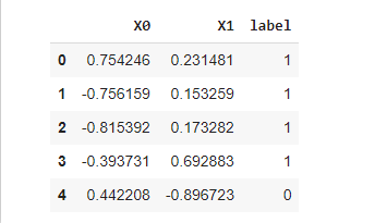
Here one question arises, what kind of labels are we dealing with?
circle.label.value_counts()
>> 1    500
   0    500
   Name: label, dtype: int64
Looks like we are dealing with a binary classification problem, because we have 2 labels(0 and 1).
plt.scatter(X[:,0], X[:,1], c = y, cmap = plt.cm.RdYlBu)
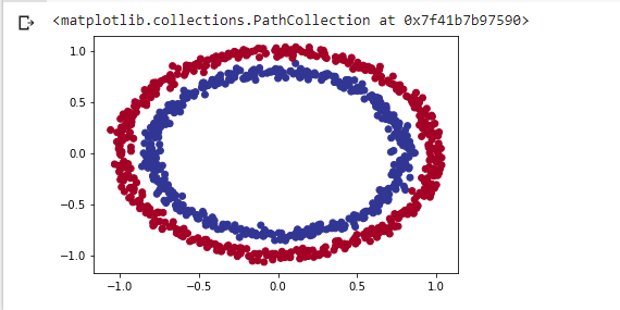
As I mentioned above, the best way of getting one with the data is visualization. Now plot says itself that what kind of model we need to build. We will build a model which is able to distinguish blue dots from red dots.
Before building any neural network model, we must check the shapes of our input and output features. they must be the same!
print(X.shape, y.shape)
print(len(X), len(y))
>> (1000, 2) (1000,)
   1000 1000
We have the same amount of values for each feature, but the shape of X is different? Why? Let’s check it out.
X[0], y[0]
>> (array([0.75424625, 0.23148074]), 1)
Okay, we have 2 X features for 1 y. So we can move forward without any problem.
Steps in Modeling Neural Network For Classification with Tensorflow
In TensorFlow there are fixed stages for creating a model:
- Creating a model – piece together the layers of a Neural Network using the Functional or Sequential API
- Compiling a model – defining how a model’s performance should be measured, and how it should improve (loss function and optimizer)
- Fitting a model – letting a model find patterns in the data
We will be using the Sequential API. So, let’s get started
tf.random.set_seed(42)
model_1 = tf.keras.Sequential([tf.keras.layers.Dense(1)])
model_1.compile(loss = tf.keras.losses.BinaryCrossentropy(),
                optimizer = tf.keras.optimizers.SGD(),
#SGD stands for Stochastic Gradient Descent

                metrics = ['accuracy'])

model_1.fit(X, y, epochs = 5)
>> Epoch 1/5 32/32 [==============================] - 1s 1ms/step - loss: 2.8544 - accuracy: 0.4600
   Epoch 2/5 32/32 [==============================] - 0s 2ms/step - loss: 0.7131 - accuracy: 0.5430
   Epoch 3/5 32/32 [==============================] - 0s 2ms/step - loss: 0.6973 - accuracy: 0.5090
   Epoch 4/5 32/32 [==============================] - 0s 2ms/step - loss: 0.6950 - accuracy: 0.5010
   Epoch 5/5 32/32 [==============================] - 0s 1ms/step - loss: 0.6942 - accuracy: 0.4830
The model’s accuracy is approximately 50% which basically means the model is just guessing, let’s try to train it longer
model_1.fit(X, y, epochs = 200, verbose = 0)
#we set verbose = 0 to remove training procedure )
model_1.evaluate(X, y)
>> 32/32 [==============================] - 0s 1ms/step - loss: 0.6935 - accuracy: 0.5000
   [0.6934829950332642, 0.5]
Even after 200 epochs, it still performs like it is guessing Next step is adding more layers and training for longer.
tf.random.set_seed(42)
model_2 = tf.keras.Sequential([ tf.keras.layers.Dense(1),

                               tf.keras.layers.Dense(1)

])

model_2.compile(loss = tf.keras.losses.BinaryCrossentropy(),

                optimizer = tf.keras.optimizers.SGD(),

                metrics = ['accuracy'])

model_2.fit(X, y, epochs = 100, verbose = 0)
model_2.evaluate(X,y)
>> 32/32 [==============================] - 0s 1ms/step - loss: 0.6933 - accuracy: 0.5000
   [0.6933314800262451, 0.5]
Still, there is not even a little change, seems like something is wrong.
Improving the Neural Network For Classification model with Tensorflow
There are different ways of improving a model at different stages:
- Creating a model – add more layers, increase the number of hidden units(neurons), change the activation functions of each layer
- Compiling a model – try different optimization functions, for example use Adam() instead of SGD().
- Fitting a model – we could increase the number of epochs
Let’s try to add more neurons and try Adam optimizer
tf.random.set_seed(42)
model_3 = tf.keras.Sequential([

  tf.keras.layers.Dense(100), # add 100 dense neurons

  tf.keras.layers.Dense(10), # add another layer with 10 neurons

  tf.keras.layers.Dense(1)

])

model_3.compile(loss=tf.keras.losses.BinaryCrossentropy(),

                optimizer=tf.keras.optimizers.Adam(),

                metrics=['accuracy'])

model_3.fit(X, y, epochs=100, verbose=0)
model_3.evaluate(X,y)
>> 32/32 [==============================] - 0s 1ms/step - loss: 0.6980 - accuracy: 0.5080
   [0.6980254650115967, 0.5080000162124634]
Still not getting better! Let’s visualize the data to see what is going wrong.
Visualize the Neural Network model
To visualize our model’s predictions we’re going to create a function plot_decision_boundary() which:
- Takes in a trained model, features, and labels
- Create a meshgrid of the different X values.
- Makes predictions across the meshgrid.
- Plots the predictions with line.
Note: This function has been adapted from two resources:
def plot_decision_boundary(model, X, y):
  # Define the axis boundaries of the plot and create a meshgrid
  x_min, x_max = X[:, 0].min() - 0.1, X[:, 0].max() + 0.1
  y_min, y_max = X[:, 1].min() - 0.1, X[:, 1].max() + 0.1
  xx, yy = np.meshgrid(np.linspace(x_min, x_max, 100),
                       np.linspace(y_min, y_max, 100))
  # Create X values (we're going to predict on all of these)
  x_in = np.c_[xx.ravel(), yy.ravel()]
  # Make predictions using the trained model
  y_pred = model.predict(x_in)
  # Check for multi-class
  if len(y_pred[0]) > 1:
     print("doing multiclass classification...")
     # We have to reshape our predictions to get them ready for plotting
     y_pred = np.argmax(y_pred, axis=1).reshape(xx.shape)
  else:
     print("doing binary classifcation...")
     y_pred = np.round(y_pred).reshape(xx.shape)
  # Plot decision boundary
  plt.contourf(xx, yy, y_pred, cmap=plt.cm.RdYlBu, alpha=0.7)
  plt.scatter(X[:, 0], X[:, 1], c=y, s=40, cmap=plt.cm.RdYlBu)
  plt.xlim(xx.min(), xx.max())
  plt.ylim(yy.min(), yy.max())

 plot_decision_boundary(model_3, X, y)
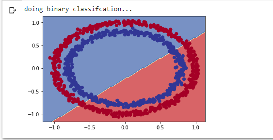
Here it is! Again visualization shows us what is wrong and what to do? Our model is trying to draw a straight line through the data, but our data is not separable by a straight line. There is something missing out on our classification problem? What it is?
This is non-linearity! We need some non-linear lines. You may get confused now, if you are thinking that you didn’t see that kind of function before, you are wrong, because you have. Let’s see them visually. Visualization always works better!
Activation Functions for Neural Networks
A = tf.cast(tf.range(-12,12), tf.float32)
print(A)
>> tf.Tensor(
   [-12. -11. -10.  -9.  -8.  -7.  -6.  -5.  -4.  -3.  -2.  -1.   0.   1.
      2.   3.   4.   5.   6.   7.   8.   9.  10.  11.], shape=(24,), dtype=float32)
Let’s see how our toy tensor looks like?
plt.plot(A)
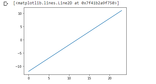
It looks like this, a straight line!
Now let’s recreate activation functions to see what they do to our tensor?
Sigmoid:
def sigmoid(x):
  return 1 / (1 + tf.exp(-x))
sigmoid(A)
plt.plot(sigmoid(A))
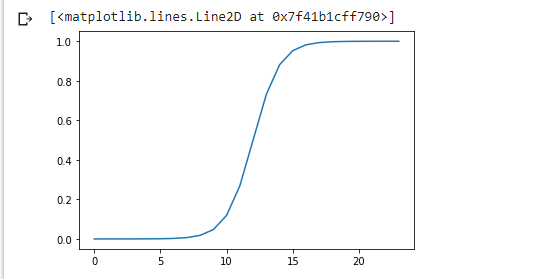
A non-straight line!
ReLu:
def relu(x):
  return tf.maximum(0,x)
plt.plot(relu(A))
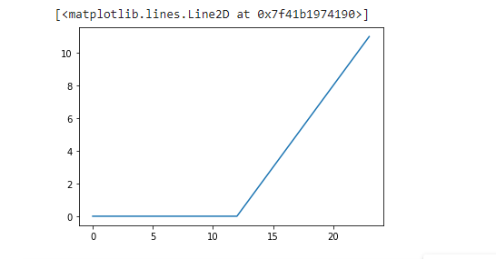
Another non-straight line!
Now you have seen non-linear activation functions, and these are what will work for us, the model cannot learn anything on a non-linear dataset with linear activation functions! If have learned this, it is time for dividing our data into training and test sets and building strong models.
X_train, y_train = X[:800], y[:800]
X_test, y_test = X[800:], y[800:]
X_train.shape, X_test.shape
>>((800, 2), (200, 2))
Great, now we’ve got training and test sets, let’s model the training data and evaluate what our model has learned on the test set.
tf.random.set_seed(42)
model_4 = tf.keras.Sequential([

                               tf.keras.layers.Dense(4, activation = 'relu'), #we may right it "tf.keras.activations.relu" too

                               tf.keras.layers.Dense(4, activation = 'relu'),

                               tf.keras.layers.Dense(1, activation = 'sigmoid')

])

model_4.compile( loss= tf.keras.losses.binary_crossentropy,

                optimizer = tf.keras.optimizers.Adam(lr = 0.01),

                metrics = ['accuracy'])

model_4.fit(X_train, y_train, epochs = 25, verbose = 0)
Evaluate the model
loss, accuracy = model_4.evaluate(X_test, y_test)
print(f' Model loss on the test set: {loss}')
print(f' Model accuracy on the test set: {100*accuracy}')
>> 7/7 [==============================] - 0s 2ms/step - loss: 0.1247 - accuracy: 1.0000
   Model loss on the test set: 0.1246885135769844
   Model accuracy on the test set: 100.0
Voila! 100% accuracy! let’s see this result visually
plt.figure(figsize=(12, 6))
plt.subplot(1, 2, 1)
plt.title("Train")
plot_decision_boundary(model_4, X=X_train, y=y_train)
plt.subplot(1, 2, 2)
plt.title("Test")
plot_decision_boundary(model_4, X=X_test, y=y_test)
plt.show()
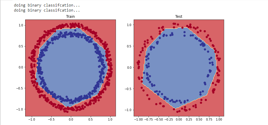
With just a few tweaks our model is now predicting the blue and red circles almost perfectly.
Conclusion
Let’s take a brief look at what we are talking about in this article. Together we looked at how to approach a classification task in the Neural Network with TensorFlow. We created 3 models in the first way that came to mind, and with the help of visualization we realized where we were wrong, we explored linearity, non-linearity, and finally, we managed to build a generalized model. What I was trying to show with all these codes and the steps I was following was that nothing is 100 percent accurate or fixed, everything continues to change every day. To guess which problem you are likely to face in which kind of data and to see which combinations lead to a better result, all you need is to write a lot more code and gain experience.
I hope the article was a little helpful to you and made some contributions.


