Long Short Term Memory (LSTM): Digging a Bit Deeper

This article was published as a part of the Data Science Blogathon.

 Introduction on Long Short Term Memory

Have you seen “Memento” or there is one Bollywood movie named “Gajni” where the hero doesn’t remember the information which occurred way back? Standard Recurrent neural networks are like the heroes of that movie, they suffer from short-term memory problems. LSTM is a special version of RNN which solves this problem of RNN through the concept of gates.

Sequence prediction problems are considered one of the most challenging problems for a long time. They include a wide range of issues from predicting the next word of the sentence to finding patterns in stock market data, from understanding movie plots to recognizing your way of speaking. As we have already discussed the basic intuition behind LSTM in my previous post (check it out on my analytics profile), it’s time we understand the nitty-gritty details behind this algorithm. We already know that LSTM works on the concept of gates. There are 3  main gates in LSTM named Forget gate, Input Gate and Output Gate.

In the previous article, we have already discussed how Long Short Term Memory solves the limitations of RNNS, in this article, we will understand all the gates in detail and will look at a simple implementation of this Algorithm.

Basic Idea Behind LSTM

Long Short Term Memory or LSTM’s are capable of learning long-term dependencies. This algorithm was first introduced by Hochreiter and Schmidhuber in 1997. LSTM work well on a wide variety of sequential problems and now they are widely used in the industry. Remembering the context of the sentence for a long period of time is their default behavior, not something they struggle to learn.

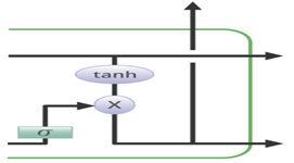
Recurrent neural networks have a very simple structure, such as a single tan-h layer:

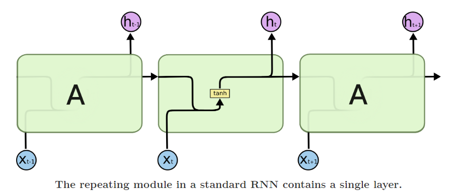
On the other hand, Long Short Term Memory  also has a chain-like structure but they are slightly different from RNN. They work on the concepts of Gate.

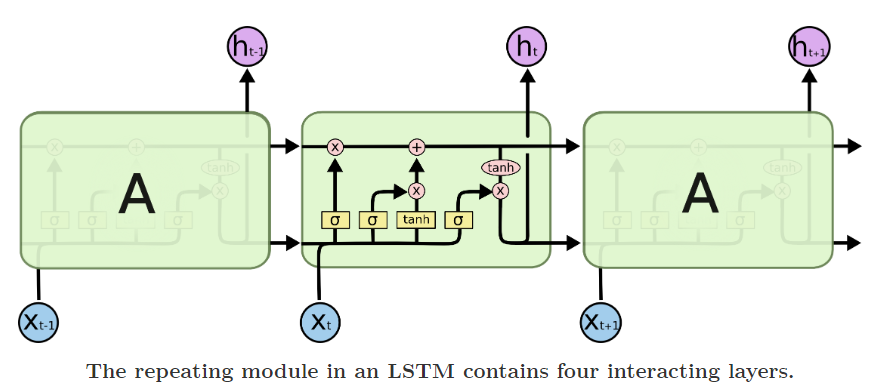
Don’t go haywire with this architecture, we will break it down into simpler steps which will make this a piece of cake to grab. LSTM has mainly 3 gates

• Forget Gate
• Input Gate
• Output Gate

Let’s look at all these gates closely and try to understand the nitty-gritty details behind all these gates.

Forget Gate

Let’s take an example of a text prediction problem.

As soon as ‘while’ is encountered, the forget gate realizes that there may be a change in the subject of the sentence or the context of the sentence. Therefore, the subject of the sentence is forgotten and the spot for the subject is vacated. When we start speaking about “Chirag” this position of the subject is allocated to “Chirag”.

All the irrelevant information is removed via the multiplication of a filter. This is necessary for optimizing the execution of the LSTM network.

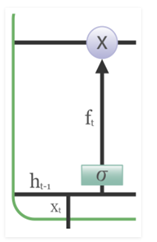
The previous hidden state H_t-1 and the current event vector X_t are joined together and multiplied with the weight matrix with an add-on of the Sigmoid activation and some bias, which generates the probability scores. Since a sigmoid activation is being applied, the output will always be 0 or 1. If the output is 0 for the particular value in the cell state, it means that forget gate wants to forget that information. Similarly, a 1 means that it wants to remember the information. Now, this vector output from the sigmoid function is multiplied by the cell state.

Here:

X_t is the current input vector

U_f is the weight associated with the input

H_t-1 is the previous hidden state

W_f is the weight associated with the hidden state

B_f is the bias added to it

If we take weight common, then this formula can be written as:

Now let’s look at the equation of memory cell state which is:

If you see here the forget gate is multiplied by the cell state of the previous timestamp and this is an element-wise multiplication. Whenever we have 1 in the forget gate matrix it will retain the value and whenever we have 0 in the forget gate then it will eliminate that information. Let’s take an example:

Whenever our model sees Mr. Watson, it will retain that information or that context in the cell state C₁ . Now C will be a matrix, right? So some of its value will retain the information that we have Mr. Watson here and now the forget gate will not allow the information to change and that is why the information will retain throughout. In RNN this information would have changed quickly as our model sees the next word. Now when we encounter some other word let’s say Ms. Mary then now the forget gate will forget the information of Mr. Watson and will add the information of Ms. Mary. This adding of new information is done by another gate known as the Input gate which we will study next.

Input Gate

To get the intuition behind this let’s take another example:

Here the important information is that “Prince” was feeling nauseous and that’s why he couldn’t enjoy the party. The fact that he told all this over the phone is not important and can be ignored. This technique of adding some new knowledge/information can be done via the input gate. It is basically used to quantify the importance of the new information carried by the input.

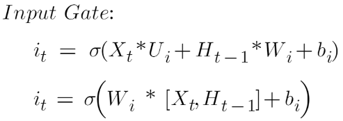
The equation of the Input gate is:

Here:

X_t is the current input vector at timestamp t

U_i is the weight matrix associated with the input

H_t-1 is the previous hidden state

W_i is the weight associated with the hidden state

b_i is the bias added to it

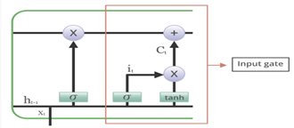
If we take weight common, then this formula can be written as:

Now we need to understand the candidate’s value. Let’s look at the memory cell state equation again:

Where <!– [if gte msEquation 12]>Ct<![endif]–> is the candidate value represented by:

The equation of candidate value is very similar to the simple recurrent neural network. This candidate value will be responsible for adding new information and as its name suggest “Candidate value” that it’s a candidate value which means potential new information we can add, and that potential new information will be filtered by this input gate.

Since we are using the sigmoid activation function in the input gate, we know that the output of the input gate will be in the range of 0-1, and thus it will filter out what new information to add since the candidate value has tan-h activation function that means its value will range between 1 and -1. If the value is negative, then the information is subtracted from the cell state and if it is positive then the information is added to the cell state at the current timestamp. Let’s take an example.

Now clearly instead of ‘her’, it should be ‘his’, and in place of ‘was,’ it should be ‘will’ because if we look at the context, the reader is talking about the future. So whenever our model reaches this word “tomorrow” it also needs to add that information along with whatever information it had before. So this is an example where we do not need to forget anything but we are just adding new information while retaining the useful information that we had before thus this model has the capacity to retain the old information for a long time along with adding information.

Output Gate

Not all the information flowing through the memory cell state is fit for being output. Let’s visualize this with an example:

In this sentence, there could be a number of outputs for the blank space. If a human being read this phrase, then he would guess that the last word ‘brave’ is an adjective that is used to describe a noun, and hence he/she will guess that the answer must be a noun. Thus, the appropriate output for this blank would be ‘Bob’.

The job of selecting useful information from the memory cell state is done via the output gate. Let’s have a look at the equation of the output gate:

Where U_o and W_o are the weights assigned to the input vector and hidden state respectively. The value of the output gate is also between 0 and 1 since we are using the sigmoid activation function. To calculate the hidden state we will use the output gate and memory cell state:

Where O_t is the matrix of output gate and C_t is the cell state matrix.

The overall architecture of LSTM looks like this:

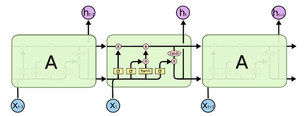
You must be wondering how these gates get to know which information to forget and which to add, and the answers lie in the weight matrices. Remember that we will train this model and after training the values of these weights will be updated in such a way that it will build a certain level of understanding, which means that after training our model will develop an understanding of which information is useful and which information is irrelevant and this understanding is built by looking at thousands and thousands of data.

An Implementation is Necessary

Let’s build a model that can predict some n number of characters after the original text of Macbeth. The original text can be found here. A revised edition of the .txt file can be found here.

We will use the library Keras library, which is a high-level API for neural networks and works on top of TensorFlow. Okay, so let’s generate some text!

Importing Libraries

# Importing dependencies numpy and keras
import numpy
from keras.models import Sequential
from keras.layers import Dense
from keras.layers import Dropout
from keras.layers import LSTM
from keras.utils import np_utils

Loading Text File

#load text
filename = "macbeth.txt"
text = (open(filename).read()).lower()
# mapping characters with integers
unique_chars = sorted(list(set(text)))
char_to_int = {}
int_to_char = {}
for i, c in enumerate (unique_chars):
    char_to_int.update({c: i})
    int_to_char.update({i: c})

In the above code, we read the ‘.txt’ file from our system. In unique_chars we have all the unique characters in the text. In char_to_int all the unique characters in the text have been assigned a number since the computer can not understand the word so we need to convert it into machine language. This is done to make the computation part easier

Preparing the Dataset

#preparing input and output dataset 
X = []
Y = []
for i in range(0,n-50,1):
    sequence = text[I:i+50]
    label = text[i+50]
    X.append([char_to_int[char] for char in s])
    Y.append(char_to_int[label])

We will prepare our model in such a way that if we want to predict ‘O’ in ‘HELLO’ then we would feel [‘H’,’E’,’L’,’L’] as input and we will get [‘O’] as an output. Similarly, here we fix the length of the window that we want (set to 50 in the example) and then save the encodings of the first 49 characters in X and the expected output i.e. the 50th character in Y.

Reshaping of X

#reshaping, normalizing and one hot encoding 
X_modified = numpy.reshape(X,(len(X),50,1))
X_modified = X_modified/float(len(ujique_chars))
Y_modified = np_utils.to_categorical(Y)

Getting the input in the correct shape is the most crucial part of this implementation. We need to understand how LSTM accepts the input, and in what shape it needs our input to be. If you check out the documentation then you would find that it takes input in [Samples, Time-steps, Features] where samples are the number of data points we have, time steps are the window size (how many words do you want to look back in order to predict the next word), features refers to the number of variables we have for the corresponding actual value in Y.

Scaling the values is a very crucial part while building a model and hence we scale the values in X_modified between 0-1 and one hot encode out true values in Y_modified.

Defining the LSTM Model

# defining the LSTM model
model = Sequential()
model.add(LSTM(300,input_shape=(X_modified.shape[1],X_modified.shape[2]),return_sequences=True))
model.add(Dropout(0.2))
model.add(LSTM(300))
model.add(Dropout(0.2))
model.add(Dense(Y_modified.shape[1],activation = 'softmax'))
model.compile(loss='categorical_crossentropy' , optimizer = 'adam)
model.summary()

In the first layer, we take 300 memory units and we also use hyperparameter return sequences which ensures that the next layer receives sequences and not just random data. Look at the hyperparameter ‘input_shape’ here I passed time-steps and a number of features and by default, it will select all the data points available. If you are still confused then please print the shape of X_modified and you’ll understand what I am trying to say. Then I am using A Dropout layer here to avoid overfitting. Lastly, we have a fully connected layer with a ‘softmax’ activation function and neurons equal to a number of unique characters.

Fitting the Model and Making Predictions

# fitting the model
model.fit(X_modified, Y_modified, epochs=200, batch_size=40)

# picking a random seed
start_index = numpy.random.randint(0, len(X)-1)
predict_string = X[start_index]

# generating characters
for i in range(50):
    x = numpy.reshape(predict_string, (1, len(predict_string), 1))
    x = x / float(len(unique_chars))

    #predicting
    pred_index = numpy.argmax(model.predict(x, verbose=0))
    char_out = int_to_char[pred_index]
    seq_in = [int_to_char[value] for value in predict_string]
    print(char_out)

    predict_string.append(pred_index)
    predict_string = predict_string[1:len(predict_string)]

The model is fit over 200 epochs, with a batch size of 40. For prediction, we are first randomly taking a start index. We put that random sentence in a variable named ‘predict_string’. We are then reshaping the new string into the shape that LSTM can accept. Finally, we are using argmax activation function to predict the next word. The prediction we get from the model gives out the char encoding of the predicted character, which means the output will be numerical so we decode it back to the character value and then append it to the pattern. Eventually, after enough training epochs, it will give better and better results over time. This is how you would use LSTM to solve a sequence prediction task.

Conclusion on Long Short Term Memory

LSTMs or Long-short term memory is a special case of RNN which tries to solve the problems faced by RNN. The problems like long-term dependencies, vanishing, and exploding gradient problems are solved by Long Short Term Memory very easily with the help of gates. It has mainly 3 gates called Forget Gate, Input Gate, and Output Gate. Forget gate is used to forget unnecessary information. The input gate is used to add new important information to the model. The output gate gives us the desired output. Apart from this 2 states are passed on to the next time stamp which is the Hidden state and the Cell state and due to this, the information isn’t updated quickly unlike RNNs.

Below are some key takeaways from the article:

• Long Short Term Memory or LSTM is used for sequential data like time series data, audio data, etc.
• Long Short Term Memory or LSTM outperforms the other models when we want our model to learn from long-term dependencies.
• It solves the problems faced by RNN (Vanishing and exploding gradient problems).
• It works on the concepts of the gate (Forget gate, Input gate, and Output gate).
• 2 states are passed on to the next time stamp which are the hidden state and cell state.
• Long Short Term Memory’s ability to forget, remember and update the information pushes it one step ahead of RNNs.

Connect with me on LinkedIn and Twitter

The media shown in this article is not owned by Analytics Vidhya and is used at the Author’s discretion.