This article was published as a part of the Data Science Blogathon
Introduction
Recurrent Neural Network (RNN) was one of the best concepts brought in that could make use of memory elements in our neural network. Before that, we had a Neural network that could perform forward propagation and backpropagate to update weights and reduce error in the network. But as we know many problems in the real world are temporal in nature and depend a lot on time.
Many language applications are always sequential and the next word in a sentence depends on the previous one. These problems were resolved using a simple RNN. But if we understand RNN we appreciate the fact that even RNN cant help us when we want to keep track of words that were earlier used in our sentence. In this article, I will discuss some of the major drawbacks of RNN and why we use a better model for most language-based applications.
Understanding Backpropagation through time (BPTT)
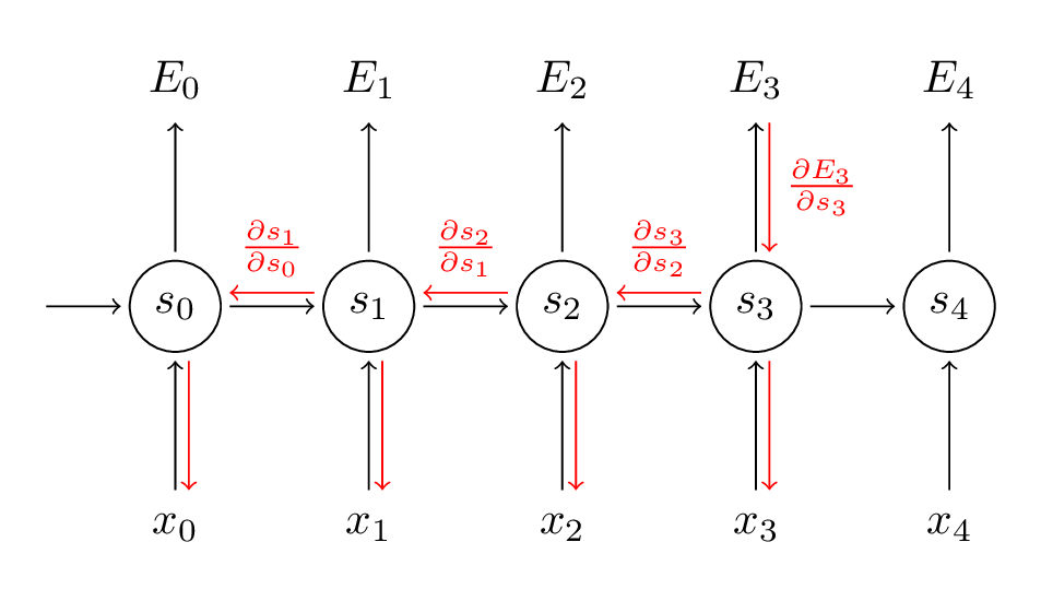
RNN uses a technique called Backpropagation through time to backpropagate through the network to adjust their weights so that we can reduce the error in the network. It got its name “through time” as in RNN we deal with sequential data and every time we go back it’s like going back in time towards the past. Here is the working of BPTT:

Source:(http://www.wildml.com/2015/10/recurrent-neural-networks-tutorial-part-3-backpropagation-through-time-and-vanishing-gradients/)
In the BPTT step, we calculate the partial derivative at each weight in the network. So if we are in time t = 3, then we consider the derivative of E3 with respect to that of S3. Now, x3 is also connected to s3. So, its derivative is also considered. Now if we see s3 is connected to s2 so s3 is depending on the value from s2 and here derivative of s3 with respect to s2 is also considered. This acts as a chain rule and we accumulate all the dependency with their derivatives and use it for error calculation.
In E3 we have a gradient that is from S3 and its equation at that time is:

Now we also have s2 associated with s3 so,

And s1 is also associated with s2 and hence now all s1,s2,s3 and having an effect on E3,

On accumulating everything we end up getting the following equation that Ws has contributed towards that network at time t=3,

The general equation for which we adjust Ws in our BPTT network can be written as,

Now as we have noticed Wx is also associated with the network. So, doing the same we can generally write,

Now that you have understood how BPTT works, this is basically all about how RNN adjusts its weights and reduces the error. Now the main fault here is this is basically only for a small network with 4 layers. But imagine if we had hundreds of layers and at a time let’s say t = 100, we would end up calculating all the partial derivatives associated with the network and this is a huge multiplication and this can bring down the overall value to a very small or minute value such that it may end up being useless to correct the error. This issue is called Vanishing Gradient Problem.
Vanishing Gradient Problem
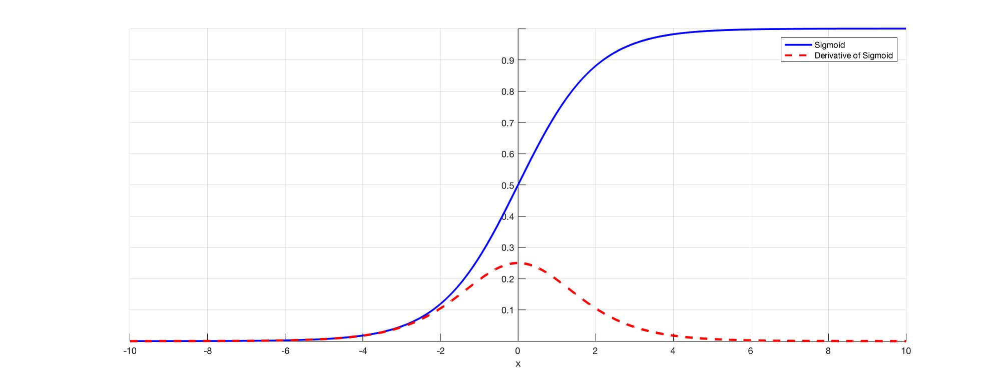
As we all know that in RNN to predict an output we will be using a sigmoid activation function so that we can get the probability output for a particular class. As we saw in the above section when we are dealing with say E3 there is a long-term dependency. The issue occurs when we are taking the derivative and derivative of the sigmoid is always below 0.25 and hence when we multiply a lot of derivatives together according to the chain rule, we end up with a vanishing value such that we cant use them for error calculation.

Source: (https://towardsdatascience.com/the-vanishing-gradient-problem-69bf08b15484)
Thus the weights and biases won’t get updated properly and as layers keep increasing we fell more into this and our model doesn’t work properly and leads to inaccuracy in the entire network.
Some ways to solve this problem is to either initialize the weight matrix properly or go for something like a ReLU instead of sigmoid or tanh functions.
Exploding Gradient Problem
Exploding gradients is a problem in which the gradient value becomes very big and this often occurs when we initialize larger weights and we could end up with NaN. If our model suffered from this issue we cannot update the weights at all. But luckily, gradient clipping is a process that we can use for this. At a pre-defined threshold value, we clip the gradient. This will prevent the gradient value to go beyond the threshold and we will never end up in big numbers or NaN.
Long term dependency of words
Now, let us consider a sentence like, “The clouds are in the ____”. Our RNN model can easily predict ‘Sky’ here and this is because of the context of clouds and it very shortly comes as an input to its previous layer. But this may not always be the case.
Image if we had a sentence like: “Jane was born in Kerala. Jane used to play for the women’s football team and has also topped at state-level examinations. Jane is very fluent in ____.”
This is a very long sentence and the issue here is as a human I can say that since Jane was born in Kerala and she had topped her state exam it’s obvious she should be very fluent in “Malayalam”. But how does our machine know about this. At the point where the model wants to predict words, it might have forgotten the context of Kerala and more about something else. This is the problem of Long term dependency in RNN.
Unidirectional in RNN
As we have discussed earlier, RNN takes data sequentially and word by word or letter by letter. Now when we are trying to predict a particular word we are not thinking about its future context. That is, let’s say we have something like: “Mouse is really good. The mouse is used to ____ for the easy use of computers.” Now if we can travel bidirectional and we can also see future context we may say ‘Scroll’ is the appropriate word here. But, if it’s unidirectional, our model has never seen computers so how does it know if we are talking about the animal mouse or computer mouse.
These problems are solved later using language models like BERT where we can input complete sentences and use the self-attention mechanism to understand the context of the text.
Use Long Short Term Memory (LSTM)
One way to solve the problem of Vanishing gradient and Long term dependency in RNN is to go for LSTM networks. LSTM has an introduction to three gates called input, output, and forget gates. In which forget gates take care of what information needs to be dropped going through the network. In this way, we can have short-term and long-term memory. We can pass the information through the network and retrieve it even at a very later stage to identify the context of prediction. The following diagram shows the LSTM network.

(https://en.wikipedia.org/wiki/Long_short-term_memory#/media/File:The_LSTM_Cell.svg)
Follow this tutorial for a better understanding and intuitive example of LSTM: https://towardsdatascience.com/illustrated-guide-to-lstms-and-gru-s-a-step-by-step-explanation-44e9eb85bf21
Hopefully, now you have understood the problems of using an RNN and why we have gone for more complex networks like LSTM.
References
1.http://www.wildml.com/2015/10/recurrent-neural-networks-tutorial-part-3-backpropagation-through-time-and-vanishing-gradients/
2. https://analyticsindiamag.com/what-are-the-challenges-of-training-recurrent-neural-networks/
3. https://towardsdatascience.com/the-vanishing-gradient-problem-69bf08b15484
4. https://en.wikipedia.org/wiki/Long_short-term_memory
5. https://www.udacity.com/course/deep-learning-nanodegree–nd101
6. Preview Image: https://unsplash.com/photos/Sot0f3hQQ4Y
Conclusion
Feel free to connect with me on:
1. https://www.linkedin.com/in/siddharth-m-426a9614a/
2. https://github.com/Siddharth1698


