This article was published as a part of the Data Science Blogathon
Overview
This article is for those who are new to GANs. The main focus would be to learn the basic theory related to Generative Adversarial Networks and practically implementing it. Maximum effort has been made to make this article simple and precise. Happy Learning!!
Introduction
You might have heard of the heated debate happening around the world about Deepfakes, if you have not heard, please watch the above video. Deepfakes is built upon a special type of neural network architecture called auto-encoders. The upgraded version of Deepfakes uses autoencoders with GANs. We won’t be going much deeper about Deepfakes, but we will explore what is happening in the GANs. The video was introduced to create a sense of interest and curiosity in the topic GANs for the readers. Before diving deep into GANs let me explain Discriminators and Generators.
Discriminators and Generators
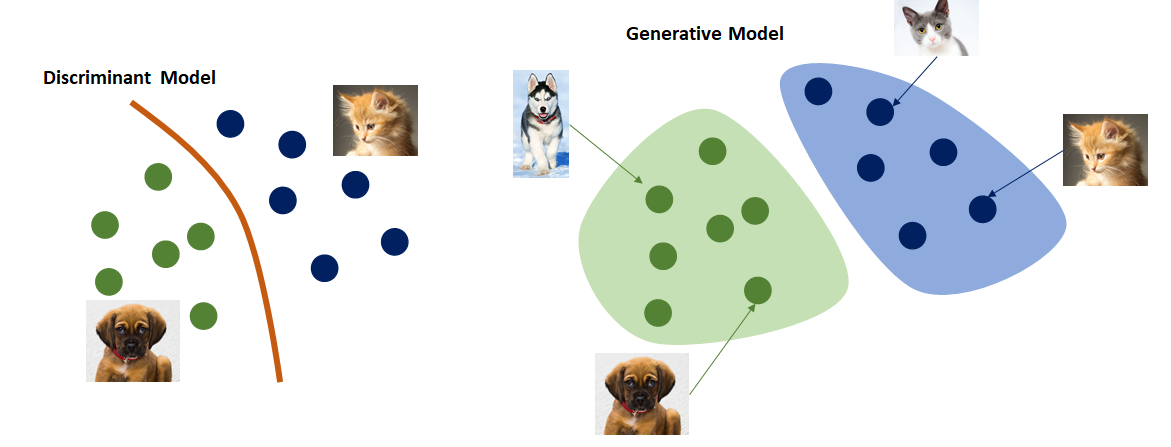
Image 1 (Link Below)
Discriminants are basically models which when fed with an input having a set of features, give the probability by which the given input will fall in a particular class. For example, Suppose that you had built a discriminative model for checking whether the given input is a cat or not? If your input is like, “the entity has fur, whiskers, claws and produces a meow sound”, then the model will say that the individual has a high probability that it belongs to the class cat, while there is a low probability of it belonging to the class dog. It basically classifies or discriminates a given input to a respective class.
Generative models are unsupervised ones and they work entirely in a different way. They are basically models from which we can draw samples or the ones that generate new data instances. Suppose that you wanted to generate a realistic image of a dog, then by using this model you will feed in random noise sometimes along with the required class, which will create a realistic image of the dog. We are using random noise in the input so that each time when the model creates a new data instance, it doesn’t create duplicates or a previously seen individual.
What’s the intuition behind GANs?
Well, intuition is really simple and understandable, it is a competition between two to win over the other. The participants in this competition are the discriminator and generator. To make you understand what the competition is, let me tell you a simple story.

Image 2 (Link Below)
The subject of our story runs around artistic paintings. There are two characters in the story, one is a forger, who makes fake copies of paintings, while the other is an art shop owner who is specialized in catching fake or duplicate copies of paintings. The forger creates fake copies of the painting and tries to sell it in the art shop. The task of the art shop owner is to detect whether the painting is fake or not. The owner is so much concerned while buying paintings from the outsiders, as he doesn’t want his shop’s credibility to go down. He always tries to upskill himself in the field of detecting fake paintings while the forger also tries to put in an increased amount of effort to outwit the shop owner.
That’s the story, now you might have understood why I had introduced you to discriminators and generators. The forger is actually the generator and the shop owner is the discriminator.
Discriminator in detail
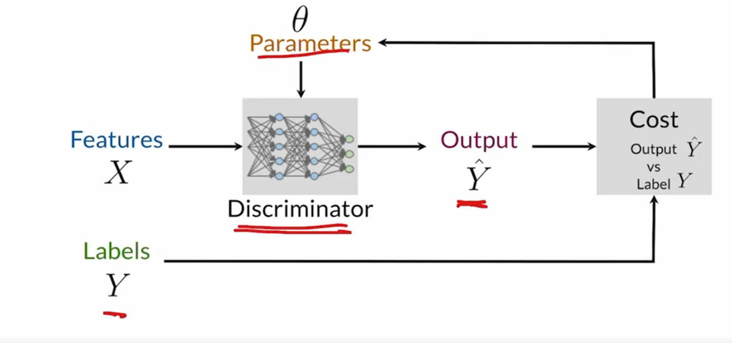
Image 3 (Link Image)
The discriminator is a fully connected neural network model which classifies the input to a particular class. There are two classes here, fake and not fake. The cost function compares the expected output and the predicted label and further, the loss is computed, and then the parameters are updated. The discriminator model wants the cost function to be minimized.
Generators in details
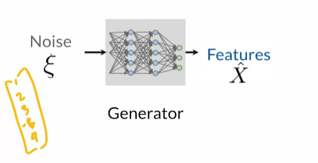
Image 4 (Link Below)
As I had told you before, generators work differently. They are fed with random noise and sometimes the class of the object that we want to generate. The model then outputs the features of the new individual belonging to the desired class. Now let’s check how the Generator learns.
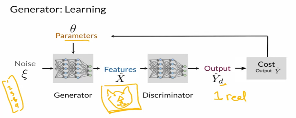
Image 5 (Link Below)
Here you can see that the features generated from the generator are fed to the discriminator and as explained before, it classifies the input as either fake or not fake. Then the generator loss is computed and further, the parameters are updated. The generator keeps feedback from the discriminator. Keep in mind that the generator wants to maximize the cost function. It wants to create maximum confusion for the discriminator. While as told before, the discriminator wants to minimize the cost function. This is kind of like a min-max competition where one competes to outperform the other.
So you might be thinking at what stage we intend to break this competition? Well, this goes on until the generator is well learned and at a particular stage, the generator outperforms the discriminator. At that point, we will freeze the parameters of the generator and use them to create samples of the desired class.
The cost function used while building a basic GAN model

Image 6 (Link Below)
I had explicitly mentioned, “Cost function used while building a basic GAN model”. This is because the BCE(Binary Cross Entropy Cost function) creates some problems such as vanishing gradient and mode collapse if the discriminator is far better compared to the generator. So as an alternative we use Wasserstein loss. As this is a beginner’s article I won’t be exploring more on that.
Code Implementation
The code is implemented using PyTorch.I had executed the code in google Colab which gives you open access to GPU for a limited time period. The dataset used here is MNIST handwritten digit dataset. We will move in a stepwise manner while explaining the code. At last, when the entire code is executed, let’s check how the Generator learns to produce more and more realistic images.
1. Importing the necessary libraries
import argparse
import os
import numpy as np
import math
import torchvision.transforms as transforms
from torchvision.utils import save_image
from torch.utils.data import DataLoader
from torchvision import datasets
from torch.autograd import Variable
import torch.nn as nn
import torch.nn.functional as F
import torch
2. Transforming and Loading the dataset
dataset = torch.utils.data.DataLoader(
    datasets.MNIST('data/', train=True, download=True,
                   transform=transforms.Compose([
                       transforms.ToTensor(),
                       transforms.Normalize((0.5,),(0.5,))
                   ])),batch_size=64, shuffle=True)
3. Making Output directory to store the images generated by Generator
os.mkdir('output')
img_shape = (1, 28, 28)
4. Creating Generator and Discriminator classes
class Discriminator(nn.Module):
    def __init__(self):
        super(Discriminator, self).__init__()
        self.fc1 = nn.Linear(28*28, 512)
        self.fc2 = nn.Linear(512, 256)
        self.fc3 = nn.Linear(256, 128)
        self.fc4 = nn.Linear(128,1)
    def forward(self, x):
        x = x.view(x.size(0),-1)
        x = F.leaky_relu( self.fc1(x),0.2)
        x = F.leaky_relu(self.fc2(x),0.2)
        x = F.leaky_relu(self.fc3(x),0.2)
        x = F.sigmoid(self.fc4(x))
        return x
# Generator
class Generator(nn.Module):
    def __init__(self):
        super(Generator, self).__init__()
        self.fc1 = nn.Linear(100, 128)
        self.fc2 = nn.Linear(128,512)
        self.fc3 = nn.Linear(512,1024 )
        self.fc4 = nn.Linear(1024,28*28)
        self.in1 = nn.BatchNorm1d(128)
        self.in2 = nn.BatchNorm1d(512)
        self.in3 = nn.BatchNorm1d(1024)
    def forward(self, x):
        x = F.leaky_relu(self.fc1(x),0.2)
        x = F.leaky_relu(self.in2(self.fc2(x)),0.2)
        x = F.leaky_relu(self.in3(self.fc3(x)),0.2)
        x = F.tanh(self.fc4(x))
        return x.view(x.shape[0],*img_shape)
5. Creating instances of Generator and Discriminator class
generator = Generator()
discriminator = Discriminator()
6. Defining the cost function
loss_func = torch.nn.BCELoss()
As explained in the theory session, we will be using the binary cross-entropy loss.
7. Moving the created instances and cost function to GPU, if available
8 Setting up the optimizer
optimizer_G = torch.optim.Adam(generator.parameters(), lr=0.0002,betas=(0.4,0.999)) # For generator
optimizer_D = torch.optim.Adam(discriminator.parameters(), lr=0.0002,betas=(0.4,0.999))# For discriminator
Tensor = torch.cuda.FloatTensor if torch.cuda.is_available() else torch.FloatTensor
9. Training the generator and discriminator
for epoch in range(20):
    for i, (imgs, _) in enumerate(dataset):
        #ground truths
        val = Tensor(imgs.size(0), 1).fill_(1.0)
        fake = Tensor(imgs.size(0), 1).fill_(0.0)
        real_imgs = imgs.cuda()
        optimizer_G.zero_grad()
        gen_input = Tensor(np.random.normal(0, 1, (imgs.shape[0],100)))
        gen = generator(gen_input)
        #generator loss gives the measure of ability to fool discriminator
        g_loss = loss_func(discriminator(gen), val)
        g_loss.backward()
        optimizer_G.step()
        optimizer_D.zero_grad()
        real_loss = loss_func(discriminator(real_imgs), val)
        fake_loss = loss_func(discriminator(gen.detach()), fake)
        d_loss = (real_loss + fake_loss) / 2
        d_loss.backward()
        optimizer_D.step()
        print ("[Epoch %d/%d] [Batch %d/%d] [D loss: %f] [G loss: %f]" % (epoch, 20, i, len(dataset),
                                                            d_loss.item(), g_loss.item()))
        total_batch = epoch * len(dataset) + i
        if total_batch % 400 == 0:
            save_image(gen.data[:25], 'output/%d.png' % total_batch, nrow=5, normalize=True)
We are setting the ground truth with the value one for the real image and zero for the generated fake image. The total loss of discriminator is taken as the average of the losses while classifying the real images as well as fake images. After every 400 batches, we are saving the generated data as images in the output directory.
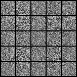
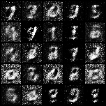
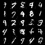
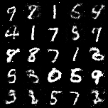
You can observe that initially the generated images were completely full of noise and in the later batches, the generator is becoming better at creating the features of the handwritten digits.
Conclusion
A brief discussion was done on the working of GANs and it’s practical implementation. If you further learn more on GANs(I have mentioned the course in the reference section), you can find more advanced architectures giving better performance than the one that we had implemented here. The entire code that was implemented is available here, please check out and explore it yourself.
References
1. Generative Adversarial Networks (GANs) Specialization –
https://www.coursera.org/specializations/generative-adversarial-networks-gans
2. Let’s implement the GANs research paper –
https://www.youtube.com/watch?v=aZpsxMZbG14
About the Author
My name is Adwait Dathan R, currently doing MTech in Artificial Intelligence and Data Science. Feel free to connect with me on Linkedin.
Image Source
- Image 1 – https://medium.com/@jordi299/about-generative-and-discriminative-models-d8958b67ad32
- Image 2 – https://www.youtube.com/watch?v=hQv8FNaJHEA
- Image 3 – https://www.coursera.org/learn/build-basic-generative-adversarial-networks-gans
- Image 4 – https://www.coursera.org/learn/build-basic-generative-adversarial-networks-gans
- Image 5 – https://www.coursera.org/learn/build-basic-generative-adversarial-networks-gans/home/welcome
- Image 6 – https://www.coursera.org/learn/build-basic-generative-adversarial-networks-gans
The media shown in this article are not owned by Analytics Vidhya and are used at the Author’s discretion.


