Introduction to Deep Learning
Artificial Intelligence, deep learning, machine learning — whatever you’re doing if you don’t understand it — learn it. Because otherwise you’re going to be a dinosaur within 3 years.
-Mark Cuban
This statement from Mark Cuban might sound drastic – but its message is spot on! We are in the middle of a revolution – a revolution caused by Big Huge data and a ton of computational power.
For a minute, think how a person would feel in the early 20th century if he/she did not understand electricity. You would have been used to doing things in a particular manner for ages and all of a sudden things around you started changing. Things which required many people can now be done with one person and electricity. We are going through a similar journey with machine learning & deep learning today.
So, if you haven’t explored or understood the power of deep learning – you should start it today. I have written this article to help you understand common terms used in deep learning.
Who should read this article?
If you are someone who wants to learn or understand deep learning, this article is meant for you. In this article, I will explain various terms used commonly in deep learning.
If you are wondering why I am writing this article – I am writing it because I want you to start your deep learning journey without hassle or without getting intimidated. When I first began reading about deep learning, there were several terms I had heard about, but it was intimidating when I tried to understand them. There are several words that are recurring when we start reading about any deep learning application.
In this article, I have created something like a deep learning dictionary for you which you can refer to whenever you need the basic definition of the most common terms used. I hope after this article these terms wouldn’t haunt you anymore.
Terms related to Deep Learning
To help you understand various terms, I have broken them into 3 different groups. If you are looking for a specific term, you can skip to that section. If you are new to the domain, I would recommend that you go through them in the order I have written them.
- Basics of Neural Networks
- Common Activation Functions
- Convolutional Neural Networks
- Recurrent Neural Networks
Basics of Neural Networks
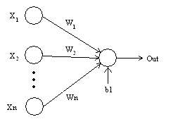
1) Neuron- Just like a neuron forms the basic element of our brain, a neuron forms the basic structure of a neural network. Just think of what we do when we get new information. When we get the information, we process it and then we generate an output. Similarly, in the case of a neural network, a neuron receives an input, processes it and generates an output that is either sent to other neurons for further processing or is the final output.
2) Weights – When input enters the neuron, it is multiplied by a weight. For example, if a neuron has two inputs, then each input will have has an associated weight assigned to it. We initialize the weights randomly and these weights are updated during the model training process. The neural network after training assigns a higher weight to the input it considers more important as compared to the ones which are considered less important. A weight of zero denotes that the particular feature is insignificant.
Let’s assume the input to be a, and the weight associated to be W1. Then after passing through the node the input becomes a*W1
3) Bias – In addition to the weights, another linear component is applied to the input, called the bias. It is added to the result of weight multiplication to the input. The bias is basically added to change the range of the weight multiplied input. After adding the bias, the result would look like a*W1+bias. This is the final linear component of the input transformation.
4) Activation Function – Once the linear component is applied to the input, a non-linear function is applied to it. This is done by applying the activation function to the linear combination. The activation function translates the input signals to output signals. The output after application of the activation function would look something like f(a*W1+b) where f() is the activation function.
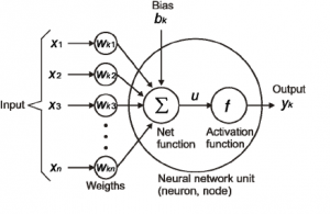
In the below diagram we have “n” inputs given as X1 to Xn and corresponding weights Wk1 to Wkn. We have a bias given as bk. The weights are first multiplied by their corresponding input and are then added together along with the bias. Let this be called as u.
u=∑w*x+b
The activation function is applied to u i.e. f(u) and we receive the final output from the neuron as yk = f(u)
Commonly applied Activation Functions
The most commonly applied activation functions are – Sigmoid, ReLU and softmax
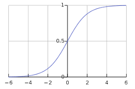
a) Sigmoid – One of the most common activation functions used is Sigmoid. It is defined as:
sigmoid(x) = 1/(1+e-x)
Source: Wikipedia
The sigmoid transformation generates a more smooth range of values between 0 and 1. We might need to observe the changes in the output with slight changes in the input values. Smooth curves allow us to do that and are hence preferred to overstep functions.
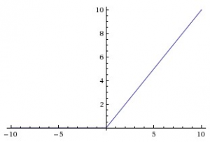
b) ReLU(Rectified Linear Units) – Instead of sigmoids, the recent networks prefer using ReLu activation functions for the hidden layers. The function is defined as:
f(x) = max(x,0).
The output of the function is X when X>0 and 0 for X<=0. The function looks like this:
source: cs231n
The major benefit of using ReLU is that it has a constant derivative value for all inputs greater than 0. The constant derivative value helps the network to train faster.
c) Softmax – Softmax activation functions are normally used in the output layer for classification problems. It is similar to the sigmoid function, with the only difference being that the outputs are normalized to sum up to 1. The sigmoid function would work in case we have a binary output, however in case we have a multiclass classification problem, softmax makes it really easy to assign values to each class which can be easily interpreted as probabilities.
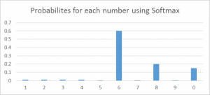
It’s very easy to see it this way – Suppose you’re trying to identify a 6 which might also look a bit like 8. The function would assign values to each number as below. We can easily see that the highest probability is assigned to 6, with the next highest assigned to 8 and so on…
5) Neural Network – Neural Networks form the backbone of deep learning. The goal of a neural network is to find an approximation of an unknown function. It is formed by interconnected neurons. These neurons have weights, and bias which is updated during the network training depending upon the error. The activation function puts a nonlinear transformation to the linear combination which then generates the output. The combinations of the activated neurons give the output.
A neural network is best defined by “Liping Yang” as –
“Neural networks are made up of numerous interconnected conceptualized artificial neurons, which pass data between themselves, and which have associated weights which are tuned based upon the network’s “experience.” Neurons have activation thresholds which, if met by a combination of their associated weights and data passed to them, are fired; combinations of fired neurons result in “learning”.
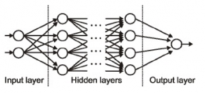
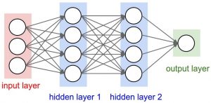
6) Input / Output / Hidden Layer – Simply as the name suggests the input layer is the one that receives the input and is essentially the first layer of the network. The output layer is the one that generates the output or is the final layer of the network. The processing layers are the hidden layers within the network. These hidden layers are the ones that perform specific tasks on the incoming data and pass on the output generated by them to the next layer. The input and output layers are the ones visible to us while being the intermediate layers are hidden.
Source: cs231n
7) MLP (Multi-Layer perceptron) – A single neuron would not be able to perform highly complex tasks. Therefore, we use stacks of neurons to generate the desired outputs. In the simplest network, we would have an input layer, a hidden layer and an output layer. Each layer has multiple neurons and all the neurons in each layer are connected to all the neurons in the next layer. These networks can also be called fully connected networks.
8) Forward Propagation – Forward Propagation refers to the movement of the input through the hidden layers to the output layers. In forward propagation, the information travels in a single direction FORWARD. The input layer supplies the input to the hidden layers and then the output is generated. There is no backward movement.
9) Cost Function – When we build a network, the network tries to predict the output as close as possible to the actual value. We measure this accuracy of the network using the cost/loss function. The cost or loss function tries to penalize the network when it makes errors.
Our objective while running the network is to increase our prediction accuracy and to reduce the error, hence minimizing the cost function. The most optimized output is the one with the least value of the cost or loss function.
If I define the cost function to be the mean squared error, it can be written as –
C= 1/m ∑(y – a)2 where m is the number of training inputs, a is the predicted value and y is the actual value of that particular example.
The learning process revolves around minimizing the cost.
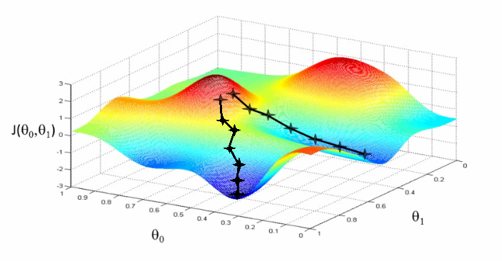
10) Gradient Descent – Gradient descent is an optimization algorithm for minimizing the cost. To think of it intuitively, while climbing down a hill you should take small steps and walk down instead of just jumping down at once. Therefore, what we do is, if we start from a point x, we move down a little i.e. delta h, and update our position to x-delta h and we keep doing the same till we reach the bottom. Consider bottom to be the minimum cost point.
Mathematically, to find the local minimum of a function one takes steps proportional to the negative of the gradient of the function.
You can go through this article for a detailed understanding of gradient descent.
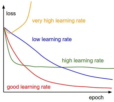
11) Learning Rate – The learning rate is defined as the amount of minimization in the cost function in each iteration. In simple terms, the rate at which we descend towards the minima of the cost function is the learning rate. We should choose the learning rate very carefully since it should neither be very large that the optimal solution is missed nor should be very low that it takes forever for the network to converge.
12) Backpropagation – When we define a neural network, we assign random weights and bias values to our nodes. Once we have received the output for a single iteration, we can calculate the error of the network. This error is then fed back to the network along with the gradient of the cost function to update the weights of the network. These weights are then updated so that the errors in the subsequent iterations is reduced. This updating of weights using the gradient of the cost function is known as back-propagation.
In back-propagation the movement of the network is backwards, the error along with the gradient flows back from the out layer through the hidden layers and the weights are updated.
13) Batches – While training a neural network, instead of sending the entire input in one go, we divide in input into several chunks of equal size randomly. Training the data on batches makes the model more generalized as compared to the model built when the entire data set is fed to the network in one go.
14) Epochs – An epoch is defined as a single training iteration of all batches in both forward and backpropagation. This means 1 epoch is a single forward and backwards pass of the entire input data.
The number of epochs you would use to train your network can be chosen by you. It’s highly likely that more number epochs would show higher accuracy of the network, however, it would also take longer for the network to converge. Also, you must take care that if the number of epochs is too high, the network might be over-fit.
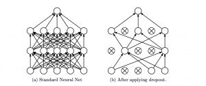
15) Dropout – Dropout is a regularization technique that prevents over-fitting of the network. As the name suggests, during training a certain number of neurons in the hidden layer is randomly dropped. This means that the training happens on several architectures of the neural network on different combinations of neurons. You can think of drop out as an ensemble technique, where the output of multiple networks is then used to produce the final output.
Source: Original paper
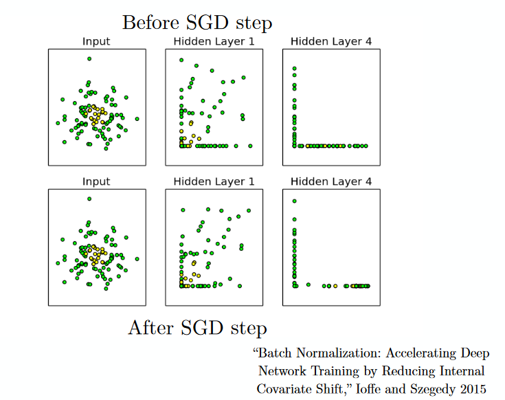
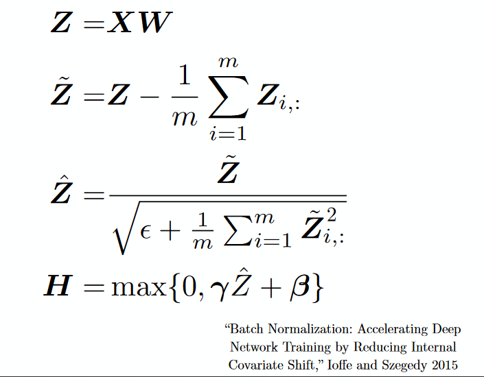
16) Batch Normalization – As a concept, batch normalization can be considered as a dam we have set as specific checkpoints in a river. This is done to ensure that the distribution of data is the same as the next layer hoped to get. When we are training the neural network, the weights are changed after each step of gradient descent. This changes how the shape of data is sent to the next layer.
But the next layer was expecting a distribution similar to what it had previously seen. So we explicitly normalize the data before sending it to the next layer.
Convolutional Neural Networks in Deep Learning
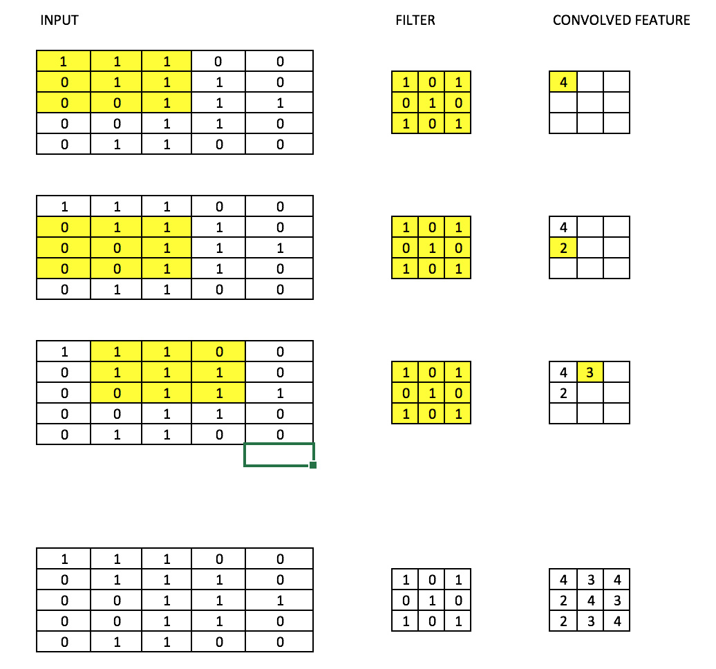
17) Filters – A filter in a CNN is like a weight matrix with which we multiply a part of the input image to generate a convoluted output. Let’s assume we have an image of size 28*28. We randomly assign a filter of size 3*3, which is then multiplied with different 3*3 sections of the image to form what is known as a convoluted output. The filter size is generally smaller than the original image size. The filter values are updated like weight values during backpropagation for cost minimization.
Consider the below image. Here filter is a 3*3 matrix 
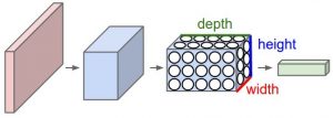
18) CNN (Convolutional neural network) – Convolutional neural networks are basically applied to image data. Suppose we have an input of size (28*28*3), If we use a normal neural network, there would be 2352(28*28*3) parameters. And as the size of the image increases the number of parameters becomes very large. We “convolve” the images to reduce the number of parameters (as shown above in filter definition). As we slide the filter over the width and height of the input volume we will produce a 2-dimensional activation map that gives the output of that filter at every position. We will stack these activation maps along the depth dimension and produce the output volume.
You can see the below diagram for a clearer picture.
Source: cs231n
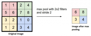
19) Pooling – It is common to periodically introduce pooling layers in between the convolution layers. This is basically done to reduce the number of parameters and prevent over-fitting. The most common type of pooling is a pooling layer of filter size(2,2) using the MAX operation. What it would do is, it would take the maximum of each 4*4 matrix of the original image.
Source: cs231n
You can also pool using other operations like Average pooling, but max-pooling has shown to work better in practice.
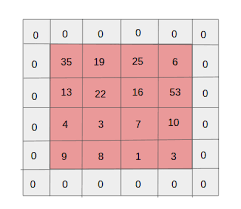
20) Padding – Padding refers to adding an extra layer of zeros across the images so that the output image has the same size as the input. This is known as the same padding.
After the application of filters, the convolved layer in the case of the same padding has a size equal to the actual image.
Valid padding refers to keeping the image as such and having all the pixels of the image which are actual or “valid”. In this case, after the application of filters, the size of the length and the width of the output keeps getting reduced at each convolutional layer.
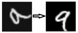
21) Data Augmentation – Data Augmentation refers to the addition of new data derived from the given data, which might prove to be beneficial for prediction. For example, it might be easier to view the cat in a dark image if you brighten it, or for instance, a 9 in the digit recognition might be slightly tilted or rotated. In this case, the rotation would solve the problem and increase the accuracy of our model. By rotating or brightening we’re improving the quality of our data. This is known as Data augmentation.
Recurrent Neural Network in Deep Learning
22) Recurrent Neuron – A recurrent neuron is one in which the output of the neuron is sent back to it for t time stamps. If you look at the diagram the output is sent back as input t times. The unrolled neuron looks like t different neurons connected together. The basic advantage of this neuron is that it gives a more generalized output.
Source: cs231n
23) RNN(Recurrent Neural Network) – Recurrent neural networks are used especially for sequential data where the previous output is used to predict the next one. In this case, the networks have loops within them. The loops within the hidden neuron give them the capability to store information about the previous words for some time to be able to predict the output. The output of the hidden layer is sent again to the hidden layer for t time stamps. The unfolded neuron looks like the above diagram. The output of the recurrent neuron goes to the next layer only after completing all the timestamps. The output sent is more generalized and the previous information is retained for a longer period.
The error is then backpropagated according to the unfolded network to update the weights. This is known as backpropagation through time(BPTT).
24) Vanishing Gradient Problem – Vanishing gradient problem arises in cases where the gradient of the activation function is very small. During backpropagation when the weights are multiplied with these low gradients, they tend to become very small and “vanish” as they go further deep in the network. This makes the neural network forget the long-range dependency. This generally becomes a problem in cases of recurrent neural networks where long term dependencies are very important for the network to remember.
This can be solved by using activation functions like ReLu which do not have small gradients.
25) Exploding Gradient Problem – This is the exact opposite of the vanishing gradient problem, where the gradient of the activation function is too large. During backpropagation, it makes the weight of a particular node very high with respect to the others rendering them insignificant. This can be easily solved by clipping the gradient so that it doesn’t exceed a certain value.
End Notes
I hope you enjoyed going through the article. I have given a high-level overview of the basic deep learning terms. I hope you now have a basic understanding of these terms. I have tried to explain everything in a language as easy as possible, however in case of any doubts/clarifications, please feel free to drop in your comments.
The media shown in this article is not owned by Analytics Vidhya and are used at the Author’s discretion.


