Improving your Deep Learning model using Model Checkpointing(Implementation)- Part 2

Introduction

In the last article, we understood the model checkpointing technique, which can be used in order to monitor the model performance after every epoch and it helps us save the best model. In this article, we’ll see how to implement that in Keras. We’ll be doing Emergency vs Non-Emergency vehicle classification using Keras. And this article is more focused on the implementation of Model checkpointing and you’re required to have a little bit of prior knowledge about creating models using Keras, as I’ve just covered those steps and not explained them in detail.

Without any further delay let’s begin!

Note: If you are more interested in learning concepts in an Audio-Visual format, We have this entire article explained in the video below. If not, you may continue reading.

So here are the steps that we’ll be following, as discussed in the previous article,  and will set up model checkpointing at the time of model training-

1. Loading the dataset

2. Pre-processing the data

3. Creating training and validation set

4. Defining the model architecture

5. Compiling the model

6. Training the model

1. Setting up model checkpointing

7. Evaluating model performance

1. Loading the dataset

Now, let’s start with the first step, which is loading the required libraries and the dataset-

# import necessary libraries and functions
import numpy as np
import pandas as pd
import matplotlib.pyplot as plt
%matplotlib inline

# importing layers from keras
from keras.layers import Dense, InputLayer
from keras.models import Sequential

# importing adam optimizer from keras optimizer module
from keras.optimizers import Adam

# train_test_split to create training and validation set
from sklearn.model_selection import train_test_split

# accuracy_score to calculate the accuracy of predictions
from sklearn.metrics import accuracy_score

So here I’ve imported the required libraries and then I’ll mount the drive-

from google.colab import drive
drive.mount('/content/drive')

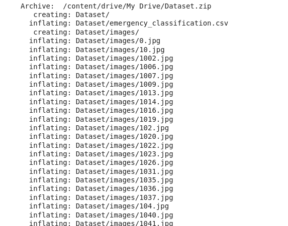
Once the drive is mounted, we’ll unzip the file-

!unzip /content/drive/My\ Drive/Dataset.zip

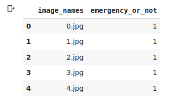
And then read the CSV file, which stores the image names, as well as the target-

# reading the csv file
data = pd.read_csv('Dataset/emergency_classification.csv')

After that set the seed value randomly and look at the first five rows of the file-

seed = 42
data.head()

So this is the file. Then we’ll use this file in order to load the images and store them in a variable name “X”, and we are separately storing the target in a variable name “y”-

# load images and store them in numpy array

# empty list to store the images
X = []

# iterating over each image
for img_name in data.image_names:

# loading the image using its name
img = plt.imread('Dataset/images/' + img_name)

# saving each image in the list
X.append(img)

# converting the list of images into array
X=np.array(X)

# storing the target variable in separate variable
y = data.emergency_or_not.values

Let’s look at the shape of our array-

# shape of the images
X.shape

So the output confirms that we have 2352 input images and each image has the shape of 224 x 224 x 3. Now the next step is to preprocess the data.

2. Pre-processing the data

So here, first of all, we are converting the three-dimensional matrix into one dimension. So we are converting the last three dimensions 224 x 224 x 3 into one dimension, which will be 224*224*3 = 150528.

# converting 3 dimensional image to 1 dimensional image
X = X.reshape(X.shape[0], 224*224*3)
X.shape

Then we’ll be checking the minimum and maximum value of the images.-

# minimum and maximum pixel values of images
X.min(), X.max()

So it’s 0 to 255. We are changing this range of 0 to 255 into 0 to 1. And we’ll normalize by dividing each of the pixel values by 255-

# normalizing the pixel values
X = X / X.max()

# minimum and maximum pixel values of images after normalizing
X.min(), X.max()

3. Creating training and validation set

Now we’ll create the training and validation set-

# shape of training and validation set
(X_train.shape, y_train.shape), (X_valid.shape, y_valid.shape)

So we have our training and validation sets are ready. Now we are going to define the architecture for our model.

4. Defining the model architecture

The input shape will be the number of features for each of these images, which will be 224*224*3. Then we have used two hidden layers each having 100 neurons and sigmoid activation function. And after that, we have our output layer, which has one neuron and the sigmoid activation function-

# defining the model architecture

model=Sequential()
model.add(InputLayer(input_shape=(224*224*3,)))
model.add(Dense(100, activation='sigmoid'))
model.add(Dense(100, activation='sigmoid'))
model.add(Dense(units=1, activation='sigmoid'))

5. Compiling the model

Next, we will compile the model where we will define the loss function as well as the optimizer.

So here we have defined the learning rate for the optimizer Adam and then we have specified loss optimizer and the metric and using model.compile we’ll compile this model-

# defining the adam optimizer and setting the learning rate as 10^-5
adam = Adam(lr=1e-5)

# compiling the model
# defining loss as binary cross-entropy
# defining optimizer as Adam
# defining metrics as accuracy

model.compile(loss='binary_crossentropy', optimizer=adam, metrics=['accuracy'])

# importing model checkpointing from keras callbacks
from keras.callbacks import ModelCheckpoint

So here I am storing the model or I would say the weights and basis of the model as best_weights.hdf5, here “.hdf5” will be the format of the file next.

# defining model checkpointing

# defining the path to store the weights
filepath="best_weights.hdf5"

As I mentioned in the last article, we have to define the metric to monitor and it’s mode so we’ll define that.

# defining the model checkpointing and metric to monitor

checkpoint = ModelCheckpoint(filepath, monitor='val_accuracy', verbose=1, save_best_only=True, mode='max')

# defining checkpointing variable
callbacks_list = [checkpoint]

So here we are calling the model checkpoint function and within this function, we have to define the path first where we wish to save the model i.e best_weights.hdf5. After that, we have to define the metric to monitor. So we are defining the metric to monitor i.e Validation Accuracy as val_accuracy. So this will monitor the validation accuracy after every epoch. Then we have “verbose = 1” so that it will print the summary after every epoch. And then we have the parameter called “save_best_only” and it is set equal to “True”, this means that it will overwrite the previously saved models and it will only save the best model. And finally, we are defining the “mode = ‘max’ “, since we want the maximum validation accuracy.

So this is how we define the model checkpoint function.

Next, we’ll train the model for 50 epochs, set the batch size to 128. Also, we’ll provide our training and validation sets. Let us run this cell.-

# training the model for 50 epochs
model_history = model.fit(X_train, y_train, epochs=50, batch_size=128, validation_data=(X_valid,y_valid), callbacks=callbacks_list)

We can see that the model training is complete and we have saved the best model at epoch number 48, after that the inaccuracy did not improve.

8. Evaluating model performance

Now that we have trained the model, let us go ahead and evaluate the model. So we are checking the accuracy scored on the validation set-

# accuracy on validation set
print('Accuracy on validation set:', accuracy_score(y_valid, model.predict_classes(X_valid)[:, 0]), '%')

So the accuracy score on the validation set comes out to be 0.7181. Now let’s load the best model-

# loading the best model
model.load_weights("best_weights.hdf5")

And once we have loaded the best model, we are going to use this in order to make the predictions and then we’ll compare how the model has performed-

# accuracy on validation set
print('Accuracy on validation set:', accuracy_score(y_valid, model.predict_classes(X_valid)[:, 0]), '%')

So we can see that the accuracy score with the best model has come out to be 0.7237, which is better than the previous validation accuracy.

So this is how we can implement model checkpointing in Keras.

End Notes

In this article, we saw the implementation of the Model Checkpointing technique on the Emergency vs Non-Emergency classification dataset.

The validation, accuracy by the model that used the weights and bias values which were stored at the last epoch was 0.71, and then when we calculated validation accuracy using our best model, it came out to be 0.72

If you are looking to kick start your Data Science Journey and want every topic under one roof, your search stops here. Check out Analytics Vidhya’s Certified AI & ML BlackBelt Plus Program

If you have any questions, let me know in the comments section!