Introduction on Perceptron Class
Deep learning is something that is ruling the markets and will continue to do for a long period of time, before starting with it we must understand what perceptron is. The origin of deep learning is often attributed to perceptron with the help of this blog you will understand how perceptron will be implemented from scratch, this will make your deep learning fundamentals very strong and robust (similar to neural nets). Alongside theory we will code also that will help us understand things very better. Here we will try to solve and see whether our perceptron will be able to solve the classical problem of AND gate (Yes, the logic gate one)
What is Perceptron?
Researchers Warren McCullock and Walter Pitts published a research paper named “a logical calculus immanent in nervous activity” where they first thought that why can’t a human brain be understood mathematically and once modelled mathematically can be learn from the surroundings and improve its performance. So right know might be little confused in the sense that whether it is possible or not. Let’s take a simple case/idea when we were born none of us knew how to walk (sad for marvel fans) but with time we learnt how to walk and now we can walk pretty well. The same idea was tried to be implemented mathematically by McCullock and Walter Pitts.
Perceptron was introduced by Frank Rosenblatt in 1957. A Perceptron is similar to artificial neural network with just one unit of neuron at the hidden layer. (It’s absolutely fine if you don’t know what artificial neural network). Let’s understand how a perceptron works and what that everything will be clear.
Let’s have a look at this image –
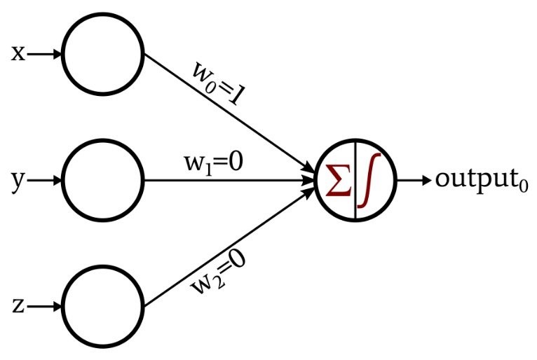
Now let’s understand each term better –
x,y,z-Inputs (Your data)
wo,w1,w2-weights (OK so how are these weights comings right??) These are initially assigned randomly and there are lot of ways to assign it but for the time being let’s stick to random technique only.
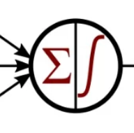
The inputs are multiplied with weights and are passed in this neuron that is perceptron activation function which in this case will help you get the outcome.
So, perceptron is used in this case when the outcome is binary and linear in nature.
Binary means you have two classes that is true or false, high or low. Linear means that you can draw a line to segregate the classes.
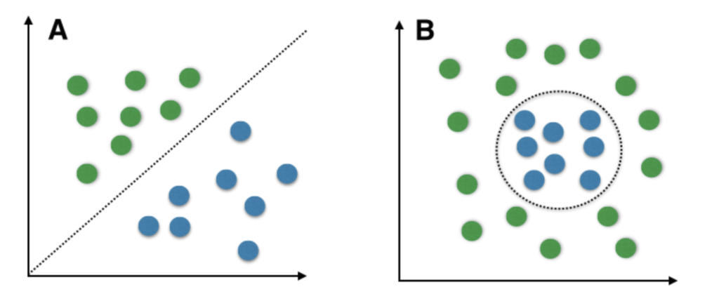
Here A is the image where the classes were linear in nature.
Here B is the image where the classes are non-linear in nature.
Now we have reached the point where the input has entered the perceptron activation function. So, what will the activation function do? It will classify whether the class is positive or negative (high or low / on or off). How? Here we have used a simple step function that will classify it as class 0 if input is negative and class 1 if the input is positive.
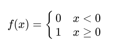
So, we have covered the forward pass of the perceptron, but what happens if we get the wrong outcome? We will learn (while walking we fall and still get up learn) similar to life neural network will also learn and correct the weights until the loss function is not minimized.
Ok so what is loss function? Here for ease, we will take the simplest loss function that is
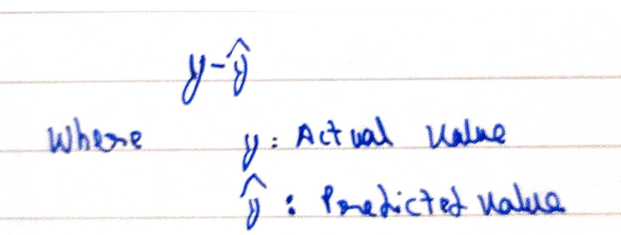
There are many loss functions. Even you can create your own loss function
This loss will get optimized with respect to the weights using the following equation
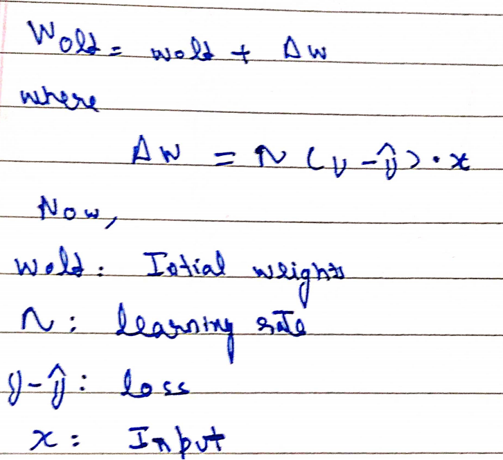
But all the calculations happen in the context of matrices and vectors so the equation in matrix space becomes:
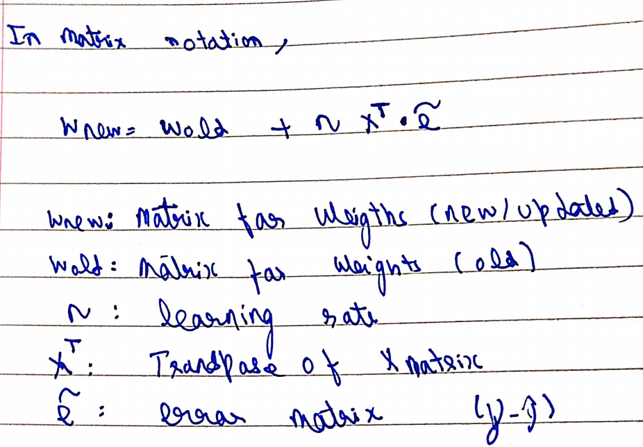
A new term eta that is learning rate has been defined. Learning rate is rate is a “tuning parameter in an optimization algorithm that determines the step size at each iteration while moving toward a minimum of a loss function”. It usually takes a value between 0 to 1.
Now in simple terms, we can understand that we will have data (that should be linear and we must try to solve a binary type classification of the problem) we pass the input into the perceptron, and using backward propagation we update the weight. Now the output depends on weights so the correct weight assignment becomes essential.
Tip – Always remember that perceptron is best used when the classes for separation are linear in nature (which is a little less often in day to day to work so that explains the evolution of deep learning). But still, it is an essential part of learning.
Summary Until Now (Interval in the show)
We have input data and we wish to classify whether the data belongs to class 1 or class 2. And the separation between the classes is linear in nature. So, we pass the data through the network, and using back-propagation weights will get updated until the loss function into consideration doesn’t become zero (in ideal case) or minimum.
I know we have discussed a lot in theory so we should move the coding implementation of the same. We will try to implement everything from scratch so that things become absolutely clear.
Before going to code, one must understand what are we trying to solve we are trying to solve the classical case of AND gate a lot of us logic gates are of no use by in the starting of evolution of deep learning logic gates very major roles, since the interpretability of the model in terms of loss function and weights is high.
And Gate
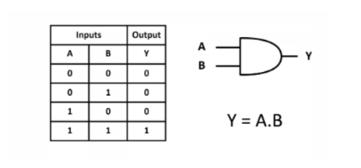
Now here the inputs will be column A and B. And the target column will be Y.
Here we will implement the model in OOPS fashion since that increases the reusability of the code
Code
import matplotlib.pyplot as plt
import numpy as np
import pandas as pd
import joblib from matplotlib.colors
import ListedColormap
plt.style.use("fivethirtyeight")

class Perceptron:
  def __init__(self, eta, epochs):
    self.weights = np.random.randn(3) * 1e-4 # RANDOM WEIGHT ASSIGNMENT
    print(f"initial weights before training: n{self.weights}")
    self.eta = eta # LEARNING RATE
    self.epochs = epochs


  def activationFunction(self, inputs, weights):
    z = np.dot(inputs, weights) # z = W * X
    return np.where(z > 0, 1, 0) # ACTIVATION FUNCTION

  def fit(self, X, y):
    self.X = X
    self.y = y

    X_with_bias = np.c_[self.X, -np.ones((len(self.X), 1))] # HERE WE ARE USING BIAS AS WELL
    print(f"X with bias: n{X_with_bias}")

    for epoch in range(self.epochs):
      print("--"*10)
      print(f"for epoch: {epoch}")
      print("--"*10)

      y_hat = self.activationFunction(X_with_bias, self.weights) # forward pass
      print(f"predicted value after forward pass: n{y_hat}")
      self.error = self.y - y_hat
      print(f"error: n{self.error}")
      self.weights = self.weights + self.eta * np.dot(X_with_bias.T, self.error)
# backward propagation
      print(f"updated weights after epoch:n{epoch}/{self.epochs} : n{self.weights}")
      print("#####"*10)


  def predict(self, X):
    X_with_bias = np.c_[X, -np.ones((len(X), 1))]
    return self.activationFunction(X_with_bias, self.weights)#Prediction function

  def total_loss(self):
    total_loss = np.sum(self.error)
    print(f"total loss: {total_loss}")
    return total_loss

def prepare_data(df):
    X=df.drop("y",axis=1)
    y=df["y"]
    return X,y
AND = {
    "x1": [0,0,1,1],
    "x2": [0,1,0,1],
    "y": [0,0,0,1],
}

df = pd.DataFrame(AND)

X,y = prepare_data(df)

ETA = 0.3 # 0 and 1
EPOCHS = 10

model = Perceptron(eta=ETA, epochs=EPOCHS)
model.fit(X, y)# Calling the function

model.total_loss()
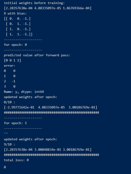
Output
Source -self
Here you can see that the loss has become zero. So our model was able to solve the problem of AND GATE. Our Model was able to learn and understand the pattern which AND gate posses.
Limitations of perceptron-
1.Gives best result when classes are linearly separable.(Which in real life is not the case)
2.Doesn’t work for XOR or related complex gate
Conclusion
In this article you got the sense of how you can implement your own perceptron class and implement it in the form of classes and object while implementing perceptron we use classes and objects since modular approach of programming makes the reusability of codes high.
Here are some of the Key learnings from this article
- What is perceptron class
- How to implement it
- Limtations of perceptron class
- Modular and OOPS approach
- Mathmatically understanding of weights and how they are updated.


