Introduction

Table of Contents
- Understanding the Data and Problem Statement
1.1 Problem Statement
1.2 Data Description - Data Analysis of Price Prediction Model
2.1 Missing Values
2.2 Handling the missing Values
2.3 Outliers
2.4 Exploratory Data Analysis
2.5 Model Development - Conclusion
Understanding the Data and Problem Statement
Problem Statement
The problem statement is to predict the sale price of a house, given the features of the house. The features are the columns in the dataset, and the target variable is the SalePrice column. The problem is a regression problem, as the target variable is continuous.
Data Description
The data description is available on Kaggle, and you can find it here. The data description contains a detailed description of each column in the dataset. The data description is very useful, as it provides a detailed description of each column in the dataset. It also provides information about the missing values in the dataset.
Data Analysis of the Price Prediction Model
Python Code:
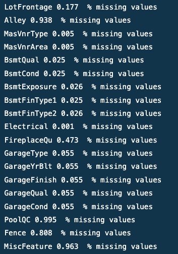
Missing Values
# Making a list of columns with missing values
missing_values = [col for col in data.columns if data[col].isnull().any()]

Output
Handling the Missing Values
# Dropping the columns with more than 15% missing values
data.drop(['Alley', 'FireplaceQu', 'PoolQC', 'Fence', 'MiscFeature'], axis=1, inplace=True)
# Filling the missing values in the remaining columns with the most frequent value
new_missing_values = [col for col in data.columns if data[col].isnull().any()]
for col in new_missing_values:
    if data[col].dtype == 'O':
        data[col].fillna(data[col].mode()[0], inplace=True)
    else:
        data[col].fillna(data[col].median(), inplace=True)
Outliers
continuous_features = [col for col in data.columns if data[col].dtype != 'O']
for col in continuous_features:
      data_copy = data.copy()
      if 0 in data_copy[col].unique():
            pass
       else:
            data_copy[col] = np.log(data_copy[col])
            data_copy['SalePrice'] = np.log(data_copy['SalePrice'])
            plt.scatter(data_copy[col], data_copy['SalePrice'])
            plt.xlabel(col)
            plt.ylabel('SalePrice')


Output
Exploratory Data Analysis
plt.figure(figsize=(10, 15))
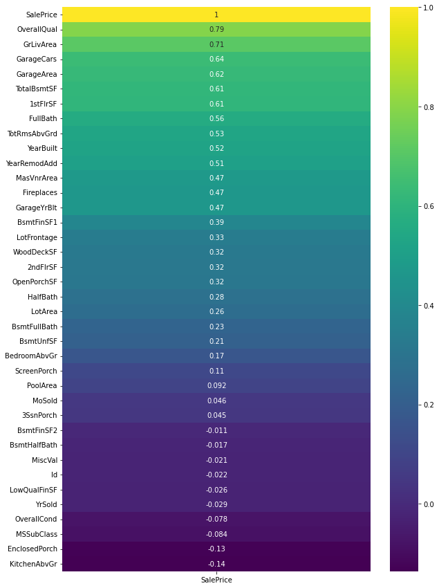
# Plotting the heatmap with respect to the correlation of the features with the target variable 'SalePrice'
sns.heatmap(data.corr()[['SalePrice']].sort_values(by='SalePrice', ascending=False), annot=True, cmap='viridis')

Output
# Regression plot between the target variable and the most correlated variables who have a correlation greater than 0.5
for col in data.corr()[data.corr()['SalePrice'] > 0.5].index:
    if col == 'SalePrice':
        pass
    else:
        sns.regplot(x=data[col], y=data['SalePrice'])
        plt.show()


Output
Model Development
# Encoding the categorical variables to the numeric datatype
from sklearn.preprocessing import LabelEncoder
for col in data.columns:
    if data[col].dtype == 'O':
        label_encoder = LabelEncoder()
        data[col] = label_encoder.fit_transform(data[col])
# Let's use Ridge Regression to build the model
from sklearn.linear_model import Ridge
from sklearn.model_selection import cross_val_score
from sklearn.metrics import mean_squared_error
# create X and y variables from Features and target variable
X = data[['OverallQual', 'GrLivArea', 'GarageCars', 'GarageArea', 'TotalBsmtSF', '1stFlrSF', 'FullBath', 'TotRmsAbvGrd', 'YearBuilt', 'YearRemodAdd']]
y = data['SalePrice']
# Function to perform ridge regression
def ridge_regression(alpha, data):
    ridge = Ridge(alpha=alpha)
    ridge.fit(X, y)
    scores = cross_val_score(ridge, X, y, scoring='neg_mean_squared_error', cv=5)
    rmse = np.sqrt(-scores)
    return rmse
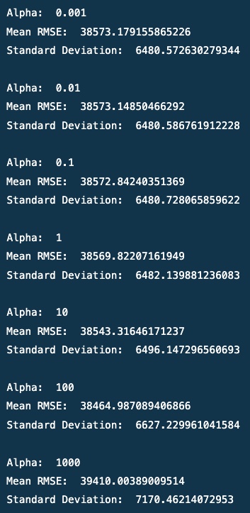
# Finding the best value of hyper-parameter of Ridge - alpha
alpha = [0.001, 0.01, 0.1, 1, 10, 100, 1000]
for i in alpha:
    print('Alpha: ', i)
    print('Mean RMSE: ', ridge_regression(i, data).mean())
    print('Standard Deviation: ', ridge_regression(i, data).std())
    print()

Output
# I will be using the ridge regression model with alpha = 100
ridge = Ridge(alpha=100)
ridge.fit(X, y)
# Loading the test data
test_data = pd.read_csv('test.csv')
# Doing all the changes that were done in the training data
test_data.drop(['Alley', 'FireplaceQu', 'PoolQC', 'Fence', 'MiscFeature'], axis=1, inplace=True)
new_missing_values = [col for col in test_data.columns if test_data[col].isnull().any()]
for col in new_missing_values:
    if test_data[col].dtype == 'O':
        test_data[col].fillna(test_data[col].mode()[0], inplace=True)
    else:
        test_data[col].fillna(test_data[col].median(), inplace=True)
# Encoding the categorical variables of test data
for col in test_data.columns:
    if test_data[col].dtype == 'O':
        label_encoder = LabelEncoder()
        test_data[col] = label_encoder.fit_transform(test_data[col])
# Selecting Features
X_test = test_data[['OverallQual', 'GrLivArea', 'GarageCars', 'GarageArea', 'TotalBsmtSF', '1stFlrSF', 'FullBath', 'TotRmsAbvGrd', 'YearBuilt', 'YearRemodAdd']]
# Predicting the target variable
y_pred = ridge.predict(X_test)
# Saving the predictions in a csv file
output = pd.DataFrame({'Id': test_data.Id, 'SalePrice': y_pred})
output.to_csv('my_submission.csv', index=False)
Conclusion
In this article, we have chosen the Ames housing dataset as the price prediction model, understand the problem statement, and perform Exploratory Data Analysis. We have also performed missing value imputation and encoding of categorical variables on the train and test data sets. Then we applied Ridge regression with different alpha values and found the best value of alpha to minimize the RMSE.
Key Takeaways:
- Three features, ‘OverallQual,’ ‘GrLivArea,’ and ‘TotalBsmtSF,’ were found to have strong positive correlations with the target variable ‘SalePrice.’
- The model performed best with alpha = 100, resulting in amses of 38464.
- The analysis showed the importance of considering multiple features in real estate price prediction models.
- Regularization techniques like Ridge regression can reduce the model’s complexity and prevent overfitting.
- The results of this project highlight the potential for using data science in real estate to make more informed decisions and improve predictions.
The media shown in this article is not owned by Analytics Vidhya and is used at the Author’s discretion.


