Introduction
In this article, we’ll cover Gradient Descent along with its variants (Mini batch Gradient Descent, SGD with Momentum).In addition to these, we’ll also discuss advanced optimizers like ADAGRAD, ADADELTA, ADAM.In this article, we’ll walk through several optimization algorithms that are used in machine learning deep learning along with its Python implementation for the same.
Table of Content:
- Need for Optimization
- Gradient Descend
- Stochastic Gradient Descent (SGD)
- Mini batch Gradient Descent (SGD)
- Momentum based Gradient Descent (SGD)
- Adagrad (short for adaptive gradient)
- Adelta
- Adam(Adaptive Gradient Descend)
- Conclusion
Need for Optimization
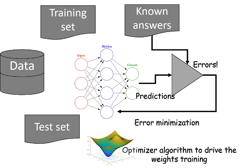
The main purpose of machine learning or deep learning is to create a model that performs well and gives accurate predictions in a particular set of cases. In order to achieve that, we machine optimization.
Optimization starts with defining some kind of loss function/cost function (objective function) and ends with minimizing it using one or the other optimization routine. The choice of an optimization algorithm can make a difference between getting a good accuracy in hours or days.
To know more about the Optimization algorithm refer to this article
1.Gradient Descent
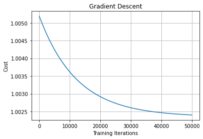
Gradient descent is one of the most popular and widely used optimization algorithms.
Gradient descent is not only applicable to neural networks but is also used in situations where we need to find the minimum of the objective function.
Python Implementation:
Note: We will be using MSE (Mean Squared Error) as the loss function.
We generate some random data points with 500 rows and 2 columns (x and y) and use them for training
data = np.random.randn(500, 2) ## Column one=X values; Column two=Y values
theta = np.zeros(2) ## Model Parameters(Weights)
Calculate the loss function using MSE
def loss_function(data,theta):
    #get m and b
    m = theta[0]
    b = theta[1]
    loss = 0
    #on each data point
    for i in range(0, len(data)):
        #get x and y
        x = data[i, 0]
        y = data[i, 1]
        #predict the value of y
        y_hat = (m*x + b)
        #compute loss as given in quation (2)
        loss = loss + ((y - (y_hat)) ** 2)
    #mean sqaured loss
    mean_squared_loss = loss / float(len(data))
    return mean_squared_loss
Calculate the Gradient of loss function for model parameters
def compute_gradients(data, theta):
    gradients = np.zeros(2)
    #total number of data points
    N = float(len(data))
    m = theta[0]
    b = theta[1]
    #for each data point
    for i in range(len(data)):
        x = data[i, 0]
        y = data[i, 1]
        #gradient of loss function with respect to m as given in (3)
        gradients[0] += - (2 / N) * x * (y - (( m* x) + b))
        #gradient of loss funcction with respect to b as given in (4)
        gradients[1] += - (2 / N) * (y - ((theta[0] * x) + b))
    #add epsilon to avoid division by zero error
    epsilon = 1e-6
    gradients = np.divide(gradients, N + epsilon)
    return gradients
theta = np.zeros(2)
gr_loss=[]
for t in range(50000):
    #compute gradients
    gradients = compute_gradients(data, theta)
    #update parameter
    theta = theta - (1e-2*gradients)
    #store the loss
    gr_loss.append(loss_function(data,theta))
2. Stochastic Gradient Descent (SGD)
In gradient descent, to perform a single parameter update, we go through all the data points in our training set. Updating the parameters of the model only after iterating through all the data points in the training set makes convergence in gradient descent very slow increases the training time, especially when we have a large dataset. To combat this, we use Stochastic Gradient Descent (SGD).
In Stochastic Gradient Descent (SGD) we don’t have to wait to update the parameter of the model after iterating all the data points in our training set instead we just update the parameters of the model after iterating through every single data point in our training set.
Since we update the parameters of the model in SGD after iterating every single data point, it will learn the optimal parameter of the model faster hence faster convergence, and this will minimize the training time as well.

3. Mini-batch Gradient Descent
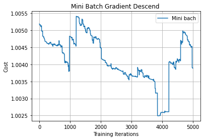
In Mini-batch gradient descent, we update the parameters after iterating some batches of data points.
Let’s say the batch size is 10, which means that we update the parameter of the model after iterating through 10 data points instead of updating the parameter after iterating through each individual data point.
Now we will calculate the loss function and update parameters
def minibatch(data, theta, lr = 1e-2, minibatch_ratio = 0.01, num_iterations = 5000):
    loss = []
    minibatch_size = int(math.ceil(len(data) * minibatch_ratio)) ## Calculate batch_size
    for t in range(num_iterations):
        sample_size = random.sample(range(len(data)), minibatch_size)
        np.random.shuffle(data)
        #sample batch of data
        sample_data = data[0:sample_size[0], :]
        #compute gradients
        grad = compute_gradients(sample_data, theta)
        #update parameters
        theta = theta - (lr * grad)
        loss.append(loss_function(data,theta))
    return loss
4.Momentum based Gradient Descent (SGD)
In order to understand the advanced variants of Gradient Descent, we need to first understand the meaning of Momentum.
The problem with Stochastic Gradient Descent (SGD) and Mini-batch Gradient Descent was that during convergence they had oscillations.
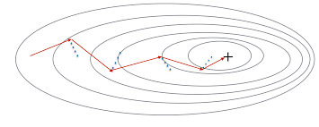
From the above plot, we can see oscillations represented with dotted lines in the case of Mini-batch Gradient Descent.
Now you must be wondering what these oscillations are?
In the case of Mini-batch Gradient Descent when we update the model parameters after iterating through all the data points in the given batch, thus the direction of the update will have some variance which leads to oscillations. Due to this oscillation, it is hard to reach convergence, and it slows down the process of attaining it. To combat this we use Momentum.
Momentum helps us in not taking the direction that does not lead us to convergence.
In other words, we take a fraction of the parameter update from the previous gradient step and add it to the current gradient step.
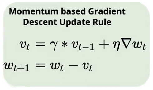
In the above equation, vt is called velocity, and it accelerates gradients in the direction that leads to convergence.
Python Implementation
def Momentum(data, theta, lr = 1e-2, gamma = 0.9, num_iterations = 5000):
    loss = []
    #Initialize vt with zeros:
    vt = np.zeros(theta.shape[0])
    for t in range(num_iterations):
        #compute gradients with respect to theta
        gradients = compute_gradients(data, theta)
        #Update vt by equation (8)
        vt = gamma * vt + lr * gradients
        #update model parameter theta by equation (9)
        theta = theta - vt
        #store loss of every iteration
        loss.append(loss_function(data,theta))
    return loss
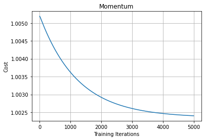
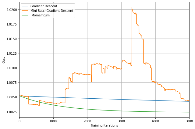
From the above plot, we can see that Momentum reduces the oscillations produced in MiniBatch Gradient Descent
5. Adagrad (short for adaptive gradient)
In the case of deep learning, we have many model parameters (Weights) and many layers to train. Our goal is to find the optimal values for all these weights.
In all of the previous methods, we observed that the learning rate was a constant value for all the parameters of the network.
However, Adagrad adaptively sets the learning rate according to a parameter hence the name adaptive gradient.

In the given equation the denominator represents the sum of the squares of the previous gradient step for the given parameter. If we can notice this denominator actually scales of learning rate.
– That is, when the sum of the squared past gradients has a high value, we are basically dividing the learning rate by a high value, so our learning rate will become less.
– Similarly, if the sum of the squared past gradients has a low value, we are dividing the learning rate by a lower value, so our learning rate value will become high.
Python Implementation
def AdaGrad(data, theta, lr = 1e-2, epsilon = 1e-8, num_iterations = 100):
    loss = []
    #initialize gradients_sum for storing sum of gradients
    gradients_sum = np.zeros(theta.shape[0])
    for t in range(num_iterations):
        #compute gradients with respect to theta
        gradients = compute_gradients(data, theta)
        #compute square of sum of gradients
        gradients_sum += gradients ** 2
        #update gradients
        gradient_update = gradients / (np.sqrt(gradients_sum + epsilon))
        #update model parameter according to equation (12)
        theta = theta - (lr * gradient_update)
        loss.append(loss_function(data,theta))
    return loss
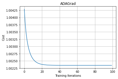
As we can see that for every iteration, we are accumulating and summing all the past squared gradients. So, on every iteration, our sum of the squared past gradients value will increase. When the sum of the squared past gradient value is high, we will have a large number in the denominator. When we divide the learning rate by a very large number, then the learning rate will become very small.
That is, our learning rate will be decreasing. When the learning rate reaches a very low value, then it takes a long time to attain convergence
6. Adadelta
We can see that in the case of Adagrad we had a vanishing learning rate problem. To deal with this we generally use Adadelta.
In Adadelta, instead of taking the sum of all the squared past gradients, we take the exponentially decaying running average or weighted average of gradients.


Python Implementation
def AdaDelta(data, theta, gamma = 0.9, epsilon = 1e-5,num_iterations = 500):
    loss = []
    #initialize running average of gradients
    E_grad2 = np.zeros(theta.shape[0])
    #initialize running average of parameter update
    E_delta_theta2 = np.zeros(theta.shape[0])
    for t in range(num_iterations):
        #compute gradients of loss with respect to theta
        gradients = compute_gradients(data, theta)
        #compute running average of gradients as given in equation (13)
        E_grad2 = (gamma * E_grad2) + ((1. - gamma) * (gradients ** 2))
        #compute delta_theta as given in equation (14)
        delta_theta = - (np.sqrt(E_delta_theta2 + epsilon)) / (np.sqrt(E_grad2 + epsilon)) * gradients
        #compute running average of parameter updates as given in equation (15)
        E_delta_theta2 = (gamma * E_delta_theta2) + ((1. - gamma) * (delta_theta ** 2))
        #update the model parameter, theta as given in equation (16)
        theta = theta + delta_theta
        #store  the loss
        loss.append(loss_function(data,theta))
    return loss
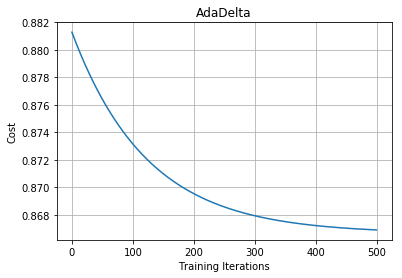
Note: The main idea behind Adadelta and RMSprop is mostly the same that is to deal with the vanishing learning rate by taking the weighted average of gradient step.
To know more about RMSprop refer to this article
7. Adam(Adaptive moment estimation)
Adam is the most widely used optimizer in deep learning. Adam takes the advantage of both RMSprop (to avoid a small learning rate) and Momentum (for fewer oscillations).
In Adam, we compute the running average of the squared gradients.
However, along with computing the running average of the squared gradients, we also
compute the running average of the gradients.

In the above equations Beta=decaying rate.

From the above equation, we can see that we are combining the equations from both Momentum and RMSProp.
Python Implementation
def Adam(data, theta, lr = 1e-2, beta1 = 0.9, beta2 = 0.9, epsilon = 1e-6, num_iterations = 1000):
    loss = []
    #initialize first moment mt
    mt = np.zeros(theta.shape[0])
    #initialize second moment vt
    vt = np.zeros(theta.shape[0])
    for t in range(num_iterations):
        #compute gradients with respect to theta
        gradients = compute_gradients(data, theta)
        #update first moment mt as given in equation (19)
        mt = beta1 * mt + (1. - beta1) * gradients
        #update second moment vt as given in equation (20)
        vt = beta2 * vt + (1. - beta2) * gradients ** 2
        #compute bias-corected estimate of mt (21)
        mt_hat = mt / (1. - beta1 ** (t+1))
        #compute bias-corrected estimate of vt (22)
        vt_hat = vt / (1. - beta2 ** (t+1))
        #update the model parameter as given in (23)
        theta = theta - (lr / (np.sqrt(vt_hat) + epsilon)) * mt_hat
        loss.append(loss_function(data,theta))
    return loss
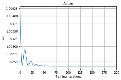
From the above plot, we can see that initially there are oscillations but as the number of iterations increases the curve becomes flatter and more smooth.
With this, we come to the end of this section. If you want all the codes in an iPython notebook format, you can download the same from my GitHub repository
Conclusion
I have found some amazing contour-based Visualizations that can further help in understanding the concept in a better way.
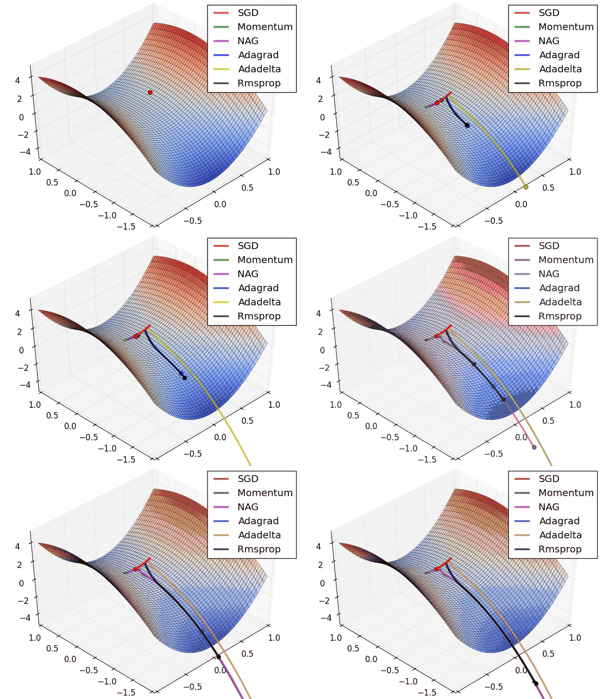
Insights from the plot:
– As we can see that SGD is the slowest to converge.
– Adagrad’s learning rate slowly becomes so small that convergence is slow.
– In the case of Adadelta and RMSprop after scaling the learning rate convergence is faster as compared to other algorithms.
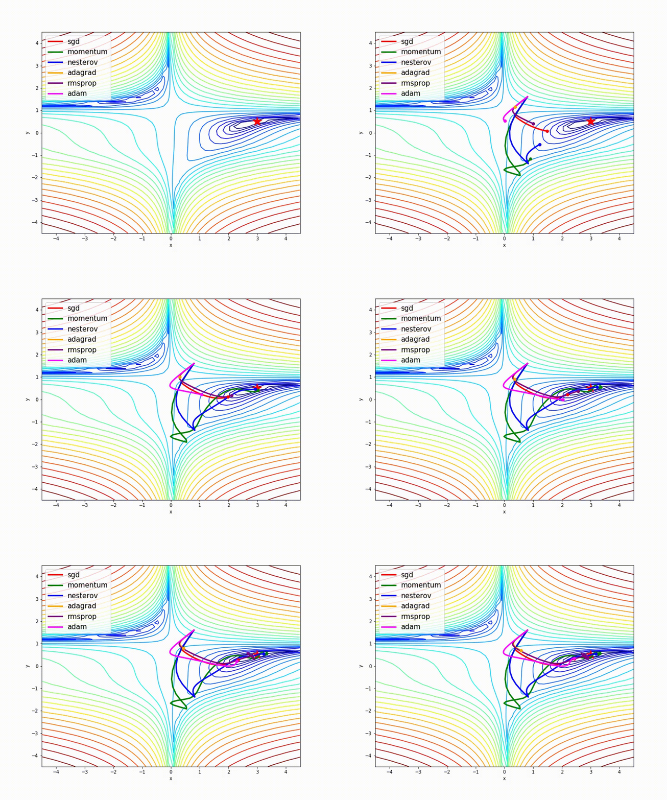
Insight from the plot:
– Momentum-based Gradient Descent generally tends to overshoot.
– Algos which scales the learning rate/ gradient-step like Adadelta and RMSprop acts as advanced SGD and is more stable in handling large gradient-step.
End Notes
In this article, we have discussed different variants of Gradient Descent and advanced optimizers which are generally used in deep learning along with Python Implementation. I recommend you can experiment more with the code and drive much more to understand more about the Optimization algorithms.
You can find the complete solution here: GitHub repository
Hope you liked this article and I hope you found it very useful in achieving what you what.
You can refer to my other article here
Dishaa Agarwal I am a data science enthusiast having knowledge in Exploratory Data Analysis, Feature Engineering, worked with multiple Machine Learning algorithms and I am currently learning Deep Learning. I always try to create content in such a way that people can easily understand the concept behind the topic.
The media shown in this article are not owned by Analytics Vidhya and are used at the Author’s discretion.


