This article was published as a part of the Data Science Blogathon
Introduction
We all heard the term graph, but what is it? Can we develop a neural network out of it, or is it just for representation? We can do all of these.
A Graph is nothing but a data structure and contains two elements inside a graph are nodes and edges.
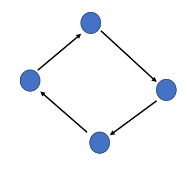
We define a graph as G = (V, E), G is indicated as a graph which is a set of V vertices or nodes and E edges. In the above image, the arrow marks are the edges the blue circles are the nodes.
Graph Neural Network is evolving day by day. It has established its importance in social networking, recommender system, many more complex problems.
What is Graph Neural Network?
Traditional CNNs cannot solve the problems related to graphs because graph data is very complex and it raises many challenges for CNNs.
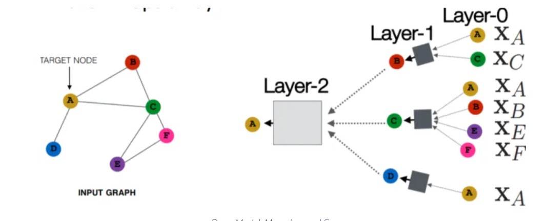
Source: https://neptune.ai/blog/graph-neural-network-and-some-of-gnn-applications
Graph Neural Network (GNN) comes under the family of Neural Networks which operates on the Graph structure and makes the complex graph data easy to understand. The basic application is node classification where every node has a label and without any ground-truth, we can predict the label for the other nodes.
Graph Neural Network (GNN) comes under the family of Neural Networks which operates on the Graph structure and makes the complex graph data easy to understand. The basic application is node classification where each and every node has a label and without any ground-truth, we can predict the label for the other nodes.
If we want to compare Convolution Neural Network and Graph Neural Network, there are many differences like designing the pipeline, loss functions, approaches, computations, etc.
Below is the one such figure from the paper “Graph neural networks: A review of methods and applications“. Consider an image for a traditional neural network, which will be like the image on the left side of the below figure, where the image is split into uniform nodes with Euclidean space between them, and on the right side of the image, we can see the nodes without Euclidean space. The uniform nodes are quite easy to compute, whereas the non-uniform nodes are called the complex structure and it is difficult to find the correlation between the nodes and is done by Graph neural network.

Implement Graph Neural Network in Python
We are going to implement GNN for the molecule Dataset. I suggest following the implementation in google Colab, as there will be no dependency issues.
First, let us check the version of PyTorch and Cuda. Also, we will get some more insights regarding the GPU in the Colab.
!python -c "import torch; print(torch.__version__)"
!python -c "import torch; print(torch.version.cuda)"
!python --version
!nvidia-smi
After you execute this in the cell you should see the output like the below image.

Here in the above image, we can see the PyTorch version, the Cuda version, and the python version running in Colab. Then we can see the GPU usage and its memory. Now we are all set to start our implementation.
First, we will start by installing RDKit, which is a collection of information regarding chemical molecules, etc.
# Install rdkit
import sys
import os
import requests
import subprocess
import shutil
from logging import getLogger, StreamHandler, INFO


logger = getLogger(__name__)
logger.addHandler(StreamHandler())
logger.setLevel(INFO)


def install(
        chunk_size=4096,
        file_name="Miniconda3-latest-Linux-x86_64.sh",
        url_base="https://repo.continuum.io/miniconda/",
        conda_path=os.path.expanduser(os.path.join("~", "miniconda")),
        rdkit_version=None,
        add_python_path=True,
        force=False):
    """install rdkit from miniconda
    ```
    import rdkit_installer
    rdkit_installer.install()
    ```
    """

    python_path = os.path.join(
        conda_path,
        "lib",
        "python{0}.{1}".format(*sys.version_info),
        "site-packages",
    )

    if add_python_path and python_path not in sys.path:
        logger.info("add {} to PYTHONPATH".format(python_path))
        sys.path.append(python_path)

    if os.path.isdir(os.path.join(python_path, "rdkit")):
        logger.info("rdkit is already installed")
        if not force:
            return

        logger.info("force re-install")

    url = url_base + file_name
    python_version = "{0}.{1}.{2}".format(*sys.version_info)

    logger.info("python version: {}".format(python_version))

    if os.path.isdir(conda_path):
        logger.warning("remove current miniconda")
        shutil.rmtree(conda_path)
    elif os.path.isfile(conda_path):
        logger.warning("remove {}".format(conda_path))
        os.remove(conda_path)

    logger.info('fetching installer from {}'.format(url))
    res = requests.get(url, stream=True)
    res.raise_for_status()
    with open(file_name, 'wb') as f:
        for chunk in res.iter_content(chunk_size):
            f.write(chunk)
    logger.info('done')

    logger.info('installing miniconda to {}'.format(conda_path))
    subprocess.check_call(["bash", file_name, "-b", "-p", conda_path])
    logger.info('done')

    logger.info("installing rdkit")
    subprocess.check_call([
        os.path.join(conda_path, "bin", "conda"),
        "install",
        "--yes",
        "-c", "rdkit",
        "python==3.7.3",
        "rdkit" if rdkit_version is None else "rdkit=={}".format(rdkit_version)])
    logger.info("done")

    import rdkit
    logger.info("rdkit-{} installation finished!".format(rdkit.__version__))


if __name__ == "__main__":
    install()
In the above program, we are importing the required modules, and defining an install function, where we will declare the necessary URL to download RDKit, chunk size, and certain functions to make sure that the kit is installed. Once you run the above code we can see the output as same as the below image.

Once the installation is complete, we can proceed with installing PyTorch geometric. This is quite complex, so go ahead and run the below code.
import torch
pytorch_version = "torch-" + torch.__version__ + ".html"
!pip install --no-index torch-scatter -f https://pytorch-geometric.com/whl/$pytorch_version
!pip install --no-index torch-sparse -f https://pytorch-geometric.com/whl/$pytorch_version
!pip install --no-index torch-cluster -f https://pytorch-geometric.com/whl/$pytorch_version
!pip install --no-index torch-spline-conv -f https://pytorch-geometric.com/whl/$pytorch_version
!pip install torch-geometric
Here we are importing torch and for the specific torch version, we are installing torch-scatter, torch-sparse, torch-cluster, torch-spline-conv, and finally torch-geometric. This will take some time to install. After the installation is done you can see the output similar to the below image.

Now lets import rdkit and load the molecule data.
import rdkit
from torch_geometric.datasets import MoleculeNet
# Load the ESOL dataset
data = MoleculeNet(root=".", name="ESOL")
data
The above code will load the ESOL dataset from MoleculeNet. After that let us explore the dataset.
print("Dataset type: ", type(data))
print("Dataset features: ", data.num_features)
print("Dataset target: ", data.num_classes)
print("Dataset length: ", data.len)
print("Dataset sample: ", data[0])
print("Sample  nodes: ", data[0].num_nodes)
print("Sample  edges: ", data[0].num_edges)

# edge_index = graph connections
# smiles = molecule with its atoms
# x = node features (32 nodes have each 9 features)
# y = labels (dimension)
The above code will print the dataset type, number of features in the data, number of classes, length of the dataset, also we are viewing a sample in the dataset and then we are printing the corresponding nodes and edges for that sample. Since we know that the graph consists of nodes and edges thus, we will get a clear picture of the dataset. Once you execute the above code we will see an output similar to the image below.

We can see that the sample which we are viewing, has a total of 32 nodes and 68 edges which is a quite complex structure. Also, we can see that the dataset sample is in smiles, for visualizing it we can convert it to rdkit molecule.
# Shape: [num_nodes, num_node_features]
data[0].x
# Shape [2, num_edges]
data[0].edge_index.t()
The above is just exploring how the data looks like. To convert the smiles to RDkit molecule, execute the below code.
#convert smiles to rdkit molecule
data[10]["smiles"]

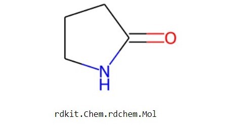
If you run the above code, it will give the molecule structure, which is confusing, hence we will visualize it in an even better way.
from rdkit import Chem
from rdkit.Chem.Draw import IPythonConsole
molecule = Chem.MolFromSmiles(data[10]["smiles"])
molecule
type(molecule)
From RDkit, we will import the Chem module, and then for visualizing it, we will call the Molecule From Smiles function which is MolFromSmiles and for this, we need to specify the data sample and the keyword “smiles” inside a list. After we execute the above code we can see the visualized molecule structure.
Lets start building our Graph Neural Network
import torch
from torch.nn import Linear
import torch.nn.functional as F
from torch_geometric.nn import GCNConv, TopKPooling, global_mean_pool
from torch_geometric.nn import global_mean_pool as gap, global_max_pool as gmp
embedding_size = 64
We will import the required modules from PyTorch and torch geometric. Now we will define our Graph Neural Network.
class GCN(torch.nn.Module):
    def __init__(self):
        # Init parent
        super(GCN, self).__init__()
        torch.manual_seed(42)

        # GCN layers
        self.initial_conv = GCNConv(data.num_features, embedding_size)
        self.conv1 = GCNConv(embedding_size, embedding_size)
        self.conv2 = GCNConv(embedding_size, embedding_size)
        self.conv3 = GCNConv(embedding_size, embedding_size)

        # Output layer
        self.out = Linear(embedding_size*2, data.num_classes)

    def forward(self, x, edge_index, batch_index):
        # First Conv layer
        hidden = self.initial_conv(x, edge_index)
        hidden = F.tanh(hidden)

        # Other Conv layers
        hidden = self.conv1(hidden, edge_index)
        hidden = F.tanh(hidden)
        hidden = self.conv2(hidden, edge_index)
        hidden = F.tanh(hidden)
        hidden = self.conv3(hidden, edge_index)
        hidden = F.tanh(hidden)

        # Global Pooling (stack different aggregations)
        hidden = torch.cat([gmp(hidden, batch_index),
                            gap(hidden, batch_index)], dim=1)

        # Apply a final (linear) classifier.
        out = self.out(hidden)

        return out, hidden
In the above code, we have created a class called GCN, in that we will create some Graph convolutional layers. For the first layer, we will give the input as the number of input features in the data, that is data.num_features, the output is the embedding size which is 64. We will declare four such layers, and the output will be a linear layer. This is our Graph neural network.
model = GCN()
print(model)
print("Number of parameters: ", sum(p.numel() for p in model.parameters()))
Initialize the model and to see the GNN layers, just print the model. After you execute the above code it will print out the layers in the model. And to see the number of parameters in the model we use a for loop to loop through the model parameters and print it.

from torch_geometric.data import DataLoader
import warnings
warnings.filterwarnings("ignore")
# Root mean squared error
loss_fn = torch.nn.MSELoss()
optimizer = torch.optim.Adam(model.parameters(), lr=0.0007)
# Use GPU for training
device = torch.device("cuda:0" if torch.cuda.is_available() else "cpu")
model = model.to(device)
We will define the loss function and here we are using mean squared error loss and Adam optimizer. And we will use GPU for training. Now let us define the Data loader to feed the data and the training function.
# Wrap data in a data loader
data_size = len(data)
NUM_GRAPHS_PER_BATCH = 64
loader = DataLoader(data[:int(data_size * 0.8)],
                    batch_size=NUM_GRAPHS_PER_BATCH, shuffle=True)
test_loader = DataLoader(data[int(data_size * 0.8):],
                         batch_size=NUM_GRAPHS_PER_BATCH, shuffle=True)

def train(data):
    for batch in loader:
      # Use GPU
      batch.to(device)
      # Reset gradients
      optimizer.zero_grad()
      # Passing the node features and the connection info
      pred, embedding = model(batch.x.float(), batch.edge_index, batch.batch)
      loss = torch.sqrt(loss_fn(pred, batch.y))
      loss.backward()
      # Update using the gradients
      optimizer.step()
    return loss, embedding

print("Starting training...")
losses = []
for epoch in range(2000):
    loss, h = train(data)
    losses.append(loss)
    if epoch % 100 == 0:
      print(f"Epoch {epoch} | Train Loss {loss}")
In the above code, we are getting the data size that is the length of the data, setting one of the hyperparameters that are the number of graphs per batch as 64. Here we are using 80% of the data for training and 20% for testing. We can see in the training data loader function data[: int(data_size * 0.8) which means that 80% of the data is for training and similarly, we do it for testing the data loader.
Then we define the train function, which takes data as input. It is a traditional neural network training function where we are initializing the batch to GPU, then resetting the gradients, and then we will pass the node features and the connection information and finally updating the Gradients. Here we are training the model for 2000 epochs and printing the loss information after every 100 Epochs. Once we run the above code, we will get the training information.
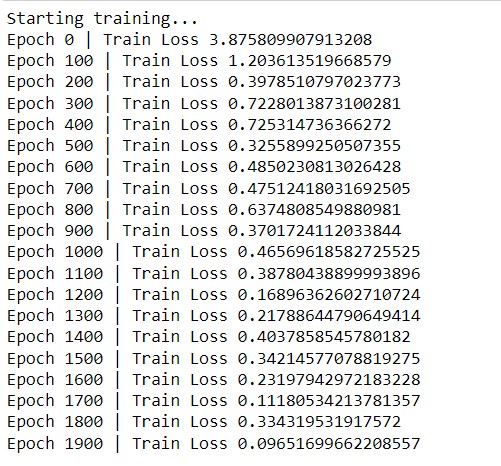
We trained the model for 2000 epochs and we can also see that the loss is gradually decreasing. After the model training is completed, we can analyze the result for one batch to see how it looks. We can convert it to a data frame to see it in a better way. For the first column, we will have the actual value and in the second column, the predicted value. So that we can see that how our model is performing.
Analyzing the Results for One Batch
import pandas as pd

# Analyze the results for one batch
test_batch = next(iter(test_loader))
with torch.no_grad():
    test_batch.to(device)
    pred, embed = model(test_batch.x.float(), test_batch.edge_index, test_batch.batch)
    df = pd.DataFrame()
    df["y_real"] = test_batch.y.tolist()
    df["y_pred"] = pred.tolist()
df["y_real"] = df["y_real"].apply(lambda row: row[0])
df["y_pred"] = df["y_pred"].apply(lambda row: row[0])
df
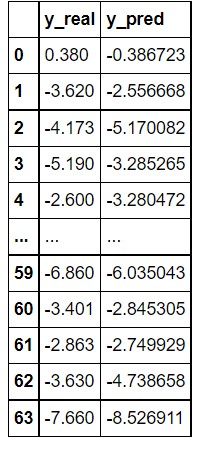
In the above image, you can see that the model has performed very well in the prediction. The predicted values are quite close to the actual value. If you want a more precise value you can play with the layers of the graph neural network and other parameters.
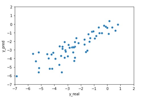
Finally, we can plot these predictions to get better visualization.
import seaborn as sns
plt = sns.scatterplot(data=df, x="y_real", y="y_pred")
plt.set(xlim=(-7, 2))
plt.set(ylim=(-7, 2))
plt
End Notes
That’s it. This is the basic implementation and an introduction to Graph Neural Network. From this, you can proceed and create your dataset to feed for the model and test it. Also, we can make it much deeper and train it with a different kind of dataset so that we can get a better picture of its working as well as its application.
Thank You


