Introduction
If there is one area in data science that has led to the growth of Machine Learning and Artificial Intelligence in the last few years, it is Deep Learning. From research labs in universities with low success in the industry to powering every smart device on the planet – Deep Learning and Neural Networks have started a revolution. And the first step of training a neural network is Forward Propagation.
Note: If you are more interested in learning concepts in an Audio-Visual format, We have this entire article explained in the video below. If not, you may continue reading.
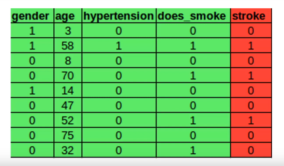
Before we start let’s have a look at a sample data set which will be used to train the neural network-
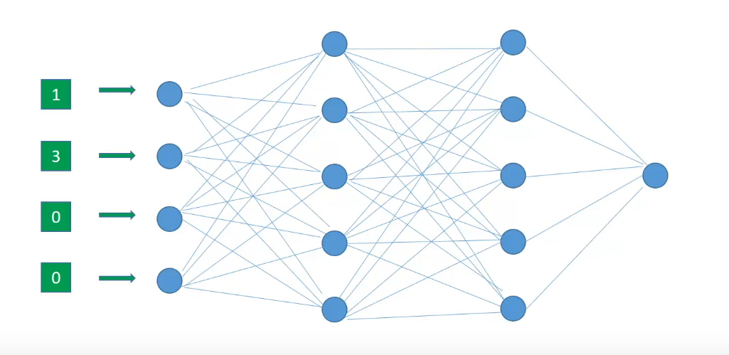
This data set has four independent features represented by green and one dependent feature represented by red. For the sake of simplicity let’s focus on the first row and try to understand forward propagation with this single row input. Each of the independent features in the first row will be passed to the input layer of the neural network to act as input.
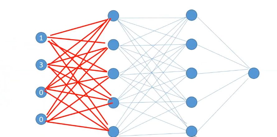
Now we start off the forward propagation by randomly initializing the weights of all neurons. These weights are depicted by the edges connecting two neurons. Hence the weights of a neuron can be more appropriately thought of as weights between two layers since edges connect two layers.
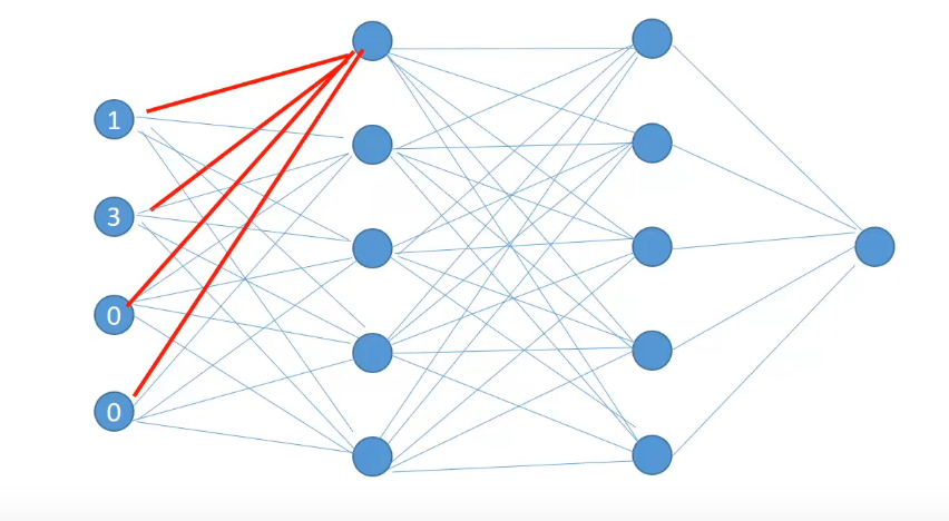
Now let’s talk about this first neuron in the first hidden layer.
This neuron receives input from all the neurons in the previous layer and combines it with its own set of weights represented by the red edges. And after applying some activation function, calculates the output known as Hidden Activation for this neuron. The output of the hidden activation will serve as input for the next layer neurons. Similarly, the hidden activations for all of the neurons in the layer are calculated.
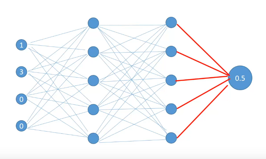
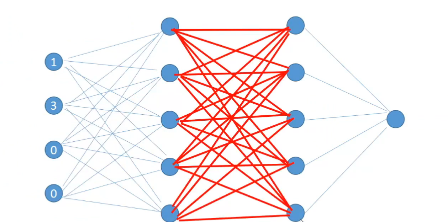
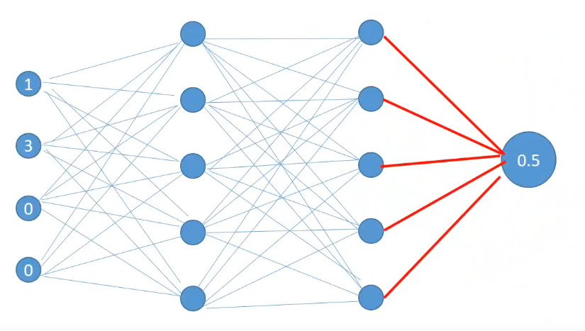
So all the activations for the first hidden layer have been calculated. These activations will serve as inputs to the layer after them. Once the hidden activations for the last hidden layer are calculated, they are combined by a final set of weights between the last hidden layer and the output layer to produce an output for a single row observation.
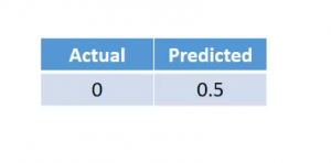
These calculations of the first row features are 0.5 and the predicted value becomes 0.5 against the actual value of 0.
Now if you notice that carefully we calculated the hidden activations for each of the neurons sequentially, that is one after the other. In fact, one optimization that we can make to the calculation is to calculate them in parallel. Since the calculation of neurons is independent of each other they can be computed in parallel easily. We can calculate the first hidden activation simultaneously-
then calculate the activation of the second layer simultaneously,
and then finally calculate the output.
This series of calculations which takes us from the input to output is called Forward Propagation.
We will now understand the error generated during the predictions and what can be the possible reasons behind those errors.
Errors in Neural Network
So far we have seen how forward propagation helps us in calculating outputs. Let’s say for a particular row the actual target is 0 and the predicted target is 0.5. We can use this predicted value to calculate the error for a particular row. The kind of error that we have chosen here is Squared Error.
There can be other error calculation formulas but for the sake of simplicity, we have chosen this one.
What can be changed to reduce error?
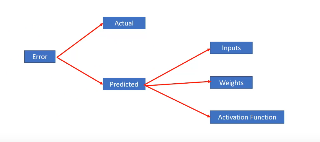
Now that we have an error what can be possible reasons for this and what can be changed to reduce errors? We know that the error is directly dependent upon two quantities- the actual values and the predicted values.
We cannot change the actual values so this is out of the possible suspects. Next, we know that the predicted values which are also the hidden activations are dependent upon 3 things-
- Inputs to the output layer i.e the hidden activation of the second layer
- Weights between the second hidden layer and the output
- And the activation function present at the output layer
We cannot directly modify the second hidden layer activations since they’re calculated at each step. So inputs are also out. We can change both the activation functions and weights but we cannot iteratively change activation functions as it would change distributions during the training time. So activation function is also out of the question.
Now, what remains are the weights between the second hidden layer and output. In fact not only can we change the weights between the second hidden layer and the output but also between the first and the second hidden layer and between the input layer and the first hidden layer. But we cannot change the weights in arbitrary amounts to check out what weights produce the lowest error as this would amount to an infinite amount of time to check what sort of weights produce the lowest error.
How to reduce Errors?
Interestingly what we can do is we can use a smart strategy to adjust the weights and reduce the errors. Specifically what we are interested is in two things-
- First is the amount of change in error on changing the weight by a small amount
- And second is the direction of that change.
End Notes
This article covered the basic idea behind the Forward Propagation and Errors in Neural Network. I hope you understood the topics well. Let me know in the comments what other topics you want me to cover.
If you are looking to kick start your Data Science Journey and want every topic under one roof, your search stops here. Check out Analytics Vidhya’s Certified AI & ML BlackBelt Plus Program
Let us know if you have any queries in the comments below.


