Introduction
Fake banknotes can easily become a problem for both small and large business enterprises. Being able to identify these banknotes when they are not genuine is very vital. This process could be time-consuming for everyday business professionals and individuals dealing with cash. This calls for a need to achieve this goal via automation. Thanks to AI, Machine Learning, and deep learning.
Consequently, we see a need to develop an Automated Machine Learning Fake banknote detection Model that can be used to detect the genuineness of these notes by even non-professionals.
This article covers a practical project where we developed a real-world prototype of how deep learning and image classification can be used in the banking sector. The goal is to complete a machine-learning demo using a real-life problem scenario. We will go from data acquisition and deep cleaning/preprocessing to simply deploying the trained model.
We will use some suitable evaluation metrics to ensure the model’s performance and how appropriately it has been learned. Since this is a banking system, we want to ensure the predictions are accurate.
This article was published as a part of the Data Science Blogathon.
Table of Contents
Problem Statement
As discussed in the introduction, it is a challenge for most individuals to distinguish between a fake banknote and a genuine one. Most people do not have any skill in this area and can get easily fooled into exchanging their good currency for fakes by scammers. We will embark on the challenge of solving this problem by using original and fake Colombian banknotes made available professionally for research.

The prerequisites to complete this project are knowledge of machine learning model pipelines, basic experience with jupyter notebooks, and an interest to take that further with deep learning. Even if this is your first experience with image processing, you do not have to worry, as every set is made simple to grasp.
Dataset Description
The dataset was made available in 2020 by the Universidad Militar Nueva Granada under CC BY 4.0 license. The dataset can be used to check systems in real-time to detect denominations and counterfeits in banknotes. The dataset is a big one in regard to size and the number of images and is made up of professionally captured images of both fake and genuine classes. Let us see the highlight below:
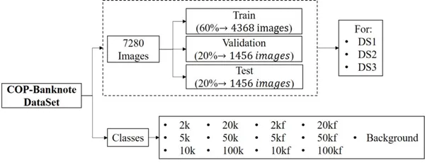
- The dataset consists of 20800 images containing 13 classes, where 6 correspond to original banknotes, another 6 to counterfeits, and 1 additional category for the background.
- It contains illumination variations, rotation, and partial views of the banknotes. Contains 3 folders each of 20800 images, corresponding to ds1, ds2, and ds3.
- Each folder contains a training, validation, and test sub-folder containing the images.
- All classes are balanced in the number of images.
Project Pipeline
In other to have a grasp of all that we will be covering, I have outlined the various steps of the model developed in detail below:
- Setting up the environment
- Importing dependencies
- Read and Load the Dataset
- Data transformation
- Data Visualization
- Tensorboarding
- Model Building
- Visualizing Predictions
- Finetuning the Convolutional Network
- Training and Evaluation
- Reporting with TensorBoard for matrices learned
- Model Testing
- Saving the trained model artifact
- Deploying locally
- Deploying to Cloud (Streamlit Cloud)
Note: To follow up practice, I recommend you reproduce this work using Google Colab, especially if you do not have a local GPU or graphic card on your computer. A challenge with deep learning is the computing environment, but thanks to Google Colab, which provides free GPU, I will show you how to engage it.
Step-1: Setting up the Environment
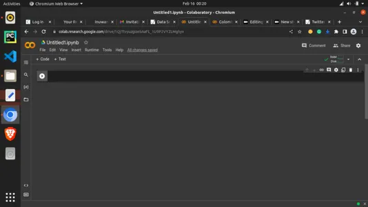
Without further ado, let us start to write some codes. We will be using Google Colab as the development environment. Now you can easily google online for Google Colaboratory or visit: https://colab.research.google.com/. It has the same interface as jupyter, so it doesn’t take much to grasp you only require a google account. The home page looks like the one below:
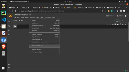
Now let us utilize the free GPU made available to use by adding it to the runtime. Click on the “Runtime” tab and select “Change runtime type,” as shown below.
Under “Hardware accelerator,” click the dropdown and select “GPU,” as shown below!
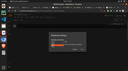
Now you have GPU connected. We can now continue with the codes.
Just before we start to import our dependencies, we need to do one last thing; getting set for our plots with matplotlib using the line below. this will help to organize outputs or graphs.
#magic function for matplotlib graphs. Graphs will be included in notebook next to the code.
%matplotlib inline
Step-2: Importing Dependencies
#importing dependencies
from __future__ import print_function, division

from datetime import datetime
from PIL import Image
import torch
import torch.nn as nn
import torch.optim as optim
from torch.optim import lr_scheduler
import numpy as np
import torchvision
from torchvision import datasets, models, transforms
from torchvision.datasets import ImageFolder
import torchvision.transforms as T
from torchvision.transforms import ToTensor
import matplotlib.pyplot as plt
import time
import os
import copy

plt.ion()   # interactive mode
Step-3: Loading of Dataset
You can find the link to the dataset at the end of this article or from the public GitHub repository that accompanies this article. After downloading the dataset, you can upload it to your google drive for easy usage. I already have it there and would just load the driver from the right column and run the cell.
from google.colab import drive
drive.mount('/content/drive')
#Dataset from drive
DATA_FILE = "/content/drive/MyDrive/MLProjects/dataset/COP"
train_dataset_location = "/content/drive/MyDrive/Datasets/dataset/COP/Train/"
val_dataset_location = "/content/drive/MyDrive/Datasets/dataset/COP/Validation/"Note: For the above snippet, you must replace the path with your own google drive file path.
Step-4: Data Transformation
#changing the format and structure of the data.
data_transforms = {
    'Train': transforms.Compose([
        transforms.Resize((224, 224)),# resizing the image dimention
        transforms.RandomHorizontalFlip(),# generating different possible image position
        transforms.ToTensor(), # tensors are like the data type for deep learning images
        transforms.Normalize([0.485, 0.456, 0.406], [0.229, 0.224, 0.225]) # normalizes the tensor image for each channel regards mean and SD
    ]),
    'Validation': transforms.Compose([
        transforms.Resize((224, 224)),
        transforms.ToTensor(),
        transforms.Normalize([0.485, 0.456, 0.406], [0.229, 0.224, 0.225])
    ]),
    'Test': transforms.Compose([
        transforms.Resize((224, 224)),
        transforms.ToTensor(),
        transforms.Normalize([0.485, 0.456, 0.406], [0.229, 0.224, 0.225])
    ]),
}

data_dir = DATA_FILE
data_types = ['Train', 'Validation', 'Test'] # grouping into the various sets
image_datasets = {x: datasets.ImageFolder(os.path.join(data_dir, x),
                                          data_transforms[x])
                  for x in data_types}
dataloaders = {x: torch.utils.data.DataLoader(image_datasets[x], batch_size=4,
                                             shuffle=True, num_workers=4)
              for x in data_types}
dataset_sizes = {x: len(image_datasets[x]) for x in data_types}
class_names = image_datasets['Train'].classes

#checking for available processor
device = torch.device("cuda:0" if torch.cuda.is_available() else "cpu")
Step-5: Data Visualization
With the help of data visualization, we can see how the data looks and what we are dealing with from the image.
# Reasigning images for visualization
image_size = 300
batch_size = 128
# converting to Tensors for visualization purpose
train_dataset = ImageFolder(data_dir+'/Train', transform=ToTensor())
val_dataset = ImageFolder(data_dir+'/Validation', transform=ToTensor())
img, label = val_dataset[13]
print(img.shape, label)
imgThe above code shows us a tensor version of one of the val_datasets at index 13.
def imshow(inp, title=None):
    """Imshow for Tensor."""
    inp = inp.numpy().transpose((1, 2, 0))
    mean = np.array([0.485, 0.456, 0.406])
    std = np.array([0.229, 0.224, 0.225])
    inp = std * inp + mean
    inp = np.clip(inp, 0, 1)
    plt.imshow(inp)
    if title is not None:
        plt.title(title)
    plt.pause(0.001)  # pause a bit so that plots are updated

# Get a batch of training data
inputs, classes = next(iter(dataloaders['Train']))

# Make a grid from batch
out = torchvision.utils.make_grid(inputs)

imshow(out, title=[class_names[x] for x in classes])
# attempting to show the image classes and directories
print("List of Directories:", os.listdir(data_dir))
classes = os.listdir(data_dir + "/Train")
print("List of classes:", classes)
List of Directories: [‘Validation,’ ‘Test,’ ‘Train’] List of classes: [‘2k’, ‘20k’, ‘50kf’, ‘20kf’, ‘5kf’, ‘Background’, ‘5k’, ‘50k’, ‘10k’, ‘10kf’, ‘100k’, ‘2kf’, ‘100kf’]
# carrying out more visualization
import matplotlib.pyplot as plt

def show_example(img, label):
    print('Label: ', train_dataset.classes[label], "("+str(label)+")")
    plt.imshow(img.permute(1, 2, 0))

import random
random_value = random.randint(1, 2000)# getting random images
show_example(*train_dataset[2000])
random_value = random.randint(1, 2000)
show_example(*train_dataset[random_value])
random_value = random.randint(1, 2000)
show_example(*train_dataset[random_value])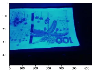
Step-6: Tensorboarding
TensorBoard is a good way of carrying out machine learning training so that you get to visualize later how the various parameters changed. It is a tool for providing the change in measurements as visualizations during the machine learning workflow. It can be seen as a type of parameter logging. We will use it here to track Loss, Accuracy, and even outliers for the last run.
CODE INPUT:
#tensorboard logging
#to track various metrics such as accuracy and log loss on training or validation set
from torch.utils.tensorboard import SummaryWriter

TB_DIR = f'runs/exp_{datetime.now().strftime("%Y%m%d-%H%M%S")}'
tb_train_writer = SummaryWriter(f'{TB_DIR}/Train')
tb_val_writer = SummaryWriter(f'{TB_DIR}/Validation')

%load_ext tensorboard
Step-7: Model Building
This is where the meat meets the cheese. Or not just yet. Let us build a helper function with all the parameters and settings we want, which we can call later.
CODE INPUT:
# helper function
def train_model(model, criterion, optimizer, scheduler, num_epochs=4):
    since = time.time()

    best_model_wts = copy.deepcopy(model.state_dict())
    best_acc = 0.0

    for epoch in range(num_epochs):
        print('Epoch {}/{}'.format(epoch, num_epochs - 1))
        print('-' * 10)

        # Each epoch has a training and validation phase
        for phase in ['Train', 'Validation']:
            if phase == 'Train':
                model.train()  # Set model to training mode
            else:
                model.eval()   # Set model to evaluate mode

            running_loss = 0.0
            running_corrects = 0

            # Iterate over data.
            for inputs, labels in dataloaders[phase]:
                inputs = inputs.to(device)
                labels = labels.to(device)

                # zero the parameter gradients
                optimizer.zero_grad()

                # forward
                # track history if only in train
                with torch.set_grad_enabled(phase == 'Train'):
                    outputs = model(inputs)
                    _, preds = torch.max(outputs, 1)
                    loss = criterion(outputs, labels)

                    # backward + optimize only if in training phase
                    if phase == 'Train':
                        loss.backward()
                        optimizer.step()

                # statistics
                running_loss += loss.item() * inputs.size(0)
                running_corrects += torch.sum(preds == labels.data)
            if phase == 'Train':
                scheduler.step()

            epoch_loss = running_loss / dataset_sizes[phase]
            epoch_acc = running_corrects.double() / dataset_sizes[phase]

            if phase == 'Train':
              tb_writer = tb_train_writer
            else:
              tb_writer = tb_val_writer

            tb_writer.add_scalar(f'Loss', epoch_loss, epoch)
            tb_writer.add_scalar(f'Accuracy', epoch_acc, epoch)

            print('{} Loss: {:.4f} Acc: {:.4f}'.format(
                phase, epoch_loss, epoch_acc))

            # deep copy the model
            if phase == 'Validation' and epoch_acc > best_acc:
                best_acc = epoch_acc
                best_model_wts = copy.deepcopy(model.state_dict())

        print()

    time_elapsed = time.time() - since
    print('Training complete in {:.0f}m {:.0f}s'.format(
        time_elapsed // 60, time_elapsed % 60))
    print('Best val Acc: {:4f}'.format(best_acc))

    tb_train_writer.close()
    tb_val_writer.close()

    # load best model weights
    model.load_state_dict(best_model_wts)
    return model
Step-8: Visualizing Predictions
We still write another helper function for making predictions. A simpler version of the code can skip this phase and just use the accuracy gotten.
CODE INPUT:
def visualize_model(model, dataset, num_images=6):
    was_training = model.training
    model.eval()
    images_so_far = 0
    fig = plt.figure()

    with torch.no_grad():
        for i, (inputs, labels) in enumerate(dataloaders[dataset]):
            inputs = inputs.to(device)
            labels = labels.to(device)

            outputs = model(inputs)
            _, preds = torch.max(outputs, 1)

            for j in range(inputs.size()[0]):
                images_so_far += 1
                ax = plt.subplot(num_images//2, 2, images_so_far)
                ax.axis('off')
                ax.set_title('predicted: {}'.format(class_names[preds[j]]))
                imshow(inputs.cpu().data[j])

                if images_so_far == num_images:
                    model.train(mode=was_training)
                    return
        model.train(mode=was_training)
Step-9: Fine-tuning the Convnet
We will load a pre-trained model and reset the final fully connected layer. this practice is known as Transfer Learning. Instead of relying on the settings we have done regarding parameters, we also decided to borrow some knowledge from the model already trained. This is a residual network known as ResNet18.
Residual Networks: Deep learning is made up of many types of Artificial Neural Networks, and Residual Neural Network is one of them.
CODE INPUT:
model_ft = models.resnet18(pretrained=True)
num_ftrs = model_ft.fc.in_features
# Here the size of each output sample is set to number of classes.
# Alternatively, it can be generalized to nn.Linear(num_ftrs, len(class_names)).
model_ft.fc = nn.Linear(num_ftrs, len(class_names))

model_ft = model_ft.to(device)

criterion = nn.CrossEntropyLoss()

# Observe that all parameters are being optimized
optimizer_ft = optim.SGD(model_ft.parameters(), lr=0.001, momentum=0.9)

# Decay LR by a factor of 0.1 every 7 epochs
exp_lr_scheduler = lr_scheduler.StepLR(optimizer_ft, step_size=7, gamma=0.1)
Step-10: Training and Evaluation
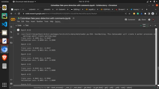
Finally, the cheese meets the meat. We now call our previous helper function and assign training parameters as we best experiment. We set the epochs to 13. Epochs are simply the rounds the training data is being looked at once as the number of iterations of all the training data. It can be seen as the number of views the training set takes around an algorithm. This definitely is important. The more it looks, the better, but we want to avoid the situation where the model looks too much. 13 epochs mean it will do so 13 times here, but you can experiment with other higher and lower values.
CODE INPUT:
# setting the number of epochs and other key parametersp
model_ft = train_model(model_ft, criterion, optimizer_ft, exp_lr_scheduler,
                       num_epochs=13)
OUTPUT:
Step-11: Showing TensorBoard for metrics learned
CODE INPUT:
# calling the tensorboard
%tensorboard --logdir='./runs'
Step-12: Saving trained Model
Lastly, we will save the model with the torch for this article.save method and the PyTorch .pt extension. Wait for a moment, then check the left column for the saved mode, right-click on it, and select download. The mode will download to your computer. This is called an artifact. We will use this artifact in the next section.
CODE INPUT:
torch.save(model_ft, 'model100.pt')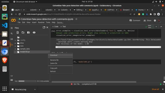
Step-13: Deploying saved Model Locally
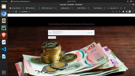
This is the fun path. We will try to see our model in real-time, making predictions with a GUI. Here we will create a python script for the Streamlit framework. The details of the code are in the GitHub repository accompanying this article. Streamlit is a lightweight framework designed for deploying machine learning frameworks locally or in the cloud. We will see the local first, then the cloud version next. Create a file and save it with the python .py extension in any code editor of your choice and write the code below.
CODE INPUT:
# importing dependencies
import io
from PIL import Image
import streamlit as st
import torch
from torchvision import transforms
import base64

# setting background
def add_bg_from_local(image_file):
    with open(image_file, "rb") as image_file:
        encoded_string = base64.b64encode(image_file.read())
    st.markdown(
    f"""
    <style>
    .stApp {{
        background-image: url(data:images/{"jpg"};base64,{encoded_string.decode()});
        background-size: cover
    }}
    </style>
    """,
    unsafe_allow_html=True
    )
add_bg_from_local('images/bg2.jpg')
# importing model
MODEL_PATH = 'model/model100.pt'
# importing class names
LABELS_PATH = 'model/model_classes.txt'

# image picker
def load_image():
    uploaded_file = st.file_uploader(label='Pick a banknote to test')
    if uploaded_file is not None:
        image_data = uploaded_file.getvalue()
        st.image(image_data)
        return Image.open(io.BytesIO(image_data))
    else:
        return None

def load_model(model_path):
    model = torch.load(model_path, map_location='cpu')
    model.eval()
    return model

def load_labels(labels_file):
    with open(labels_file, "r") as f:
        categories = [s.strip() for s in f.readlines()]
        return categories

def predict(model, categories, image):
    preprocess = transforms.Compose([
        transforms.Resize(256),
        transforms.CenterCrop(224),
        transforms.ToTensor(),
        transforms.Normalize(mean=[0.485, 0.456, 0.406], std=[0.229, 0.224, 0.225]),
    ])
    input_tensor = preprocess(image)
    input_batch = input_tensor.unsqueeze(0)

    with torch.no_grad():
        output = model(input_batch)

    probabilities = torch.nn.functional.softmax(output[0], dim=0)

    all_prob, all_catid = torch.topk(probabilities, len(categories))
    for i in range(all_prob.size(0)):
        st.write(categories[all_catid[i]], all_prob[i].item())

def main():
    st.title('Colombian Pesu banknote Detection')
    model = load_model(MODEL_PATH)
    categories = load_labels(LABELS_PATH)
    image = load_image()
    result = st.button('Predict image')
    if result:
        st.write('Checking...')
        predict(model, categories, image)

if __name__ == '__main__':
    main()
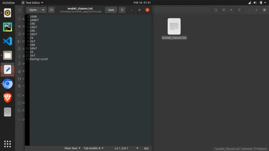
Note: the classes file imported alongside the model must be created also. To do so, create a text file named “model_classes.txt.” Save this and then download the model in a folder named “model” in the same directory as the python script. Also, you must note that the class names must be according to how they were trained. You can find this from where we printed the classes and directories above. Let every class take a single line, as the model will read the text file line after line, as shown below.
To run the python script, you must install some packages if you do not already have them. Here are the dependencies, which you can find in the repo:
- streamlit
- torch
- torchvision
After installing the dependencies, run on a terminal in the directory where your script is:
streamlit run filename.pyHopefully, this should show your app as below:
Step-14: Deploying to Cloud
Maybe you want to share your machine learning app with someone not close to you. This can be done via Cloud infrastructure. You must move your working directory to an online code management platform like GitHub to connect the repo with Streamlit Cloud. Push your directory using Git and go to https://streamlit.io/cloud with the home screen as below:

Sign up and click on “Get Started.” You will be required to sign up. It is completely free! After signing up select your GitHub repo where the app is and select it. Choose to deploy and hold on while your app bakes! Now you can copy the link for sharing.
Conclusion
We have been able to train, save and deploy a beautiful and powerful machine-learning product to the cloud using streamlit community cloud. We also got an accuracy of 100% at the 3rd epoch.
Key takeaways
- Fake banknotes can easily become a problem for the banking sector. Being able to identify these banknotes is the task we were able to achieve using deep learning.
- We developed an Automated Machine Learning Fake banknote detection Model that can be used to detect the genuineness of these notes by even non-professionals.
- We used some suitable evaluation metrics, including Loss and Accuracy, with an accuracy of 100%.
- We deployed the model both locally and on the cloud using deep learning.
References
Pachon Suescun, Cesar; Ballesteros, Dora Maria; Renza, Diego (2020), “Original and counterfeit Colombian peso banknotes”, Mendeley Data, V1, doi: 10.17632/tj8kvrbfz6.1
Links
Public GitHub repository: https://github.com/inuwamobarak/Deep-learning-in-Banking
Dataset: https://data.mendeley.com/datasets/tj8kvrbfz6/1
Streamlit: https://streamlit.io/
The media shown in this article is not owned by Analytics Vidhya and is used at the Author’s discretion.


