This article was published as a part of the Data Science Blogathon
Introduction
Covid is a deadly disease, which affects the respiratory system. It is very important to detect whether or not a person has covid. In this blog, we are going to identify whether or not a person has covid. Let’s begin this blog without any ado.
Importing
Let’s import the required tools for carrying out our task.
import pandas as pd
import numpy as np
from keras.preprocessing.image import ImageDataGenerator
from tensorflow.keras.applications import ResNet50
from tensorflow.python.keras.models import Sequential
from tensorflow.python.keras.layers import Dense, Flatten, GlobalAveragePooling2D
from tensorflow.keras.applications import ResNet50
import tensorflow as tf
import matplotlib.pyplot as plt
Reading Data
train_data=pd.read_csv("Training_set_covid.csv")
print(train_data)
| filename | label | |
|---|---|---|
| 0 | Image_1.jpg | 1 |
| 1 | Image_2.jpg | 0 |
| 2 | Image_3.jpg | 0 |
| 3 | Image_4.jpg | 0 |
| 4 | Image_5.jpg | 0 |
| … | … | … |
| 3474 | Image_3475.jpg | 0 |
| 3475 | Image_3476.jpg | 0 |
| 3476 | Image_3477.jpg | 0 |
| 3477 | Image_3478.jpg | 1 |
| 3478 | Image_3479.jpg | 0 |
Since we have just the name of the image file and their label, let’s add a column consisting of their file path. With whose help we can load images using ImageDataGenerator.
train_data["filepath"]="train/"+train_data["filename"]
print(train_data)
| filename | label | file-path | |
|---|---|---|---|
| 0 | Image_1.jpg | 1 | file-path |
| 1 | Image_2.jpg | 0 | file-path |
| 2 | Image_3.jpg | 0 | file-path |
| 3 | Image_4.jpg | 0 | file-path |
| 4 | Image_5.jpg | 0 | file-path |
| … | … | … | … |
| 3474 | Image_3475.jpg | 0 | file-path |
| 3475 | Image_3476.jpg | 0 | file-path |
| 3476 | Image_3477.jpg | 0 | file-path |
| 3477 | Image_3478.jpg | 1 | file-path |
| 3478 | Image_3479.jpg | 0 | file-path |
I have replaced the actual file path with “file-path”.
Data Augmentation
Since we have very little data, I am augmenting my data and also creating a variable where training and validation image will be stored
train_datagen=ImageDataGenerator(validation_split=0.2,zoom_range=0.2,rescale=1./255.,horizontal_flip=True)
Here, we set the zoom range to 0.2 and rescaled images to 1/255 size, and made a validation set of 20% of our training image.
train_data["label"]=train_data["label"].astype(str)
The above code will convert our int labels into string types.
Loading Images
train_images=train_datagen.flow_from_dataframe(train_data,x_col="filepath",batch_size=8,target_size=(255,255),class_mode="binary",shuffle=True,subset='training',y_col="label")
valid_images=train_datagen.flow_from_dataframe(train_data,x_col="filepath",batch_size=8,target_size=(255,255),class_mode="binary",shuffle=True,subset='validation',y_col="label")
Here, we are creating 2 data streams, 1 training set, and another validation set. For which we have set some parameters. Parameters like:
1) Batch Size –> 8
2) Target Size (Image size) –> (255,255)
3) Shuffle –> True
4) Class Mode –> Binary
As we have only 2 target attributes we have set our class mode Binary. Resnet50 takes (255,255) as input shape, hence our image size. Shuffle is set to be True, to shuffle images well enough so that both sets have various images.
RESNET50
Let’s load our ResNet50 Model. But before going into the code path, visit this site to understand what ResNet50 is and how it works.
base_model = ResNet50(input_shape=(225, 225,3), include_top=False, weights="imagenet")
for layer in base_model.layers:
    layer.trainable = False

base_model = Sequential()
base_model.add(ResNet50(include_top=False, weights='imagenet', pooling='max'))
base_model.add(Dense(1, activation='sigmoid'))
base_model.compile(optimizer = tf.keras.optimizers.SGD(lr=0.0001), loss = 'binary_crossentropy', metrics = ['acc'])
base_model.summary()
Let’s understand this code block.
First, we will load a base model with our input shape, and weights. Here, we have used image-net weight. We have removed the top as we will add our output layer.
Then, We set all our base model layers Non-Trainable as we don’t want to overwrite weights that we have imported while loading.
Now, we are creating our base model, where we add a Dense layer of 50 units to create a fully connected layer that is connected to our output dense layer with 1 unit and Sigmoid as an activation function. Then we compiled it with an SGD optimizer and some fine-tuning and binary cross-entropy as loss function.
This is how our model looks:
Model: "sequential_1"
_________________________________________________________________
Layer (type)                 Output Shape              Param #
=================================================================
resnet50 (Functional)        (None, 2048)              23587712
_________________________________________________________________
dense_1 (Dense)              (None, 1)                 2049
=================================================================
Total params: 23,589,761
Trainable params: 23,536,641
Non-trainable params: 53,120
_________________________________________________________________
Training
resnet_history = base_model.fit(train_images, validation_data = valid_images, steps_per_epoch =int(train_images.n/8), epochs = 20)
Let’s train our model with, train images, and validate them using a validation set. With 20 epochs, and steps per epochs are set to the number of train sample/8 to balance, batch size of 8.
Epoch 1/20
348/348 [==============================] - 162s 453ms/step - loss: 0.7703 - acc: 0.8588 - val_loss: 1.2608 - val_acc: 0.8791
Epoch 2/20
348/348 [==============================] - 84s 242ms/step - loss: 0.3550 - acc: 0.9198 - val_loss: 2.8488 - val_acc: 0.4518
Epoch 3/20
348/348 [==============================] - 84s 241ms/step - loss: 0.3501 - acc: 0.9229 - val_loss: 1.0196 - val_acc: 0.7007
Epoch 4/20
348/348 [==============================] - 84s 241ms/step - loss: 0.3151 - acc: 0.9207 - val_loss: 0.5498 - val_acc: 0.8633
Epoch 5/20
348/348 [==============================] - 85s 245ms/step - loss: 0.2376 - acc: 0.9281 - val_loss: 0.4247 - val_acc: 0.9094
Epoch 6/20
348/348 [==============================] - 86s 246ms/step - loss: 0.2273 - acc: 0.9248 - val_loss: 0.3911 - val_acc: 0.8978
Epoch 7/20
348/348 [==============================] - 86s 248ms/step - loss: 0.2166 - acc: 0.9319 - val_loss: 0.2936 - val_acc: 0.9295
Epoch 8/20
348/348 [==============================] - 87s 251ms/step - loss: 0.2016 - acc: 0.9389 - val_loss: 0.3025 - val_acc: 0.9281
Epoch 9/20
348/348 [==============================] - 87s 249ms/step - loss: 0.1557 - acc: 0.9516 - val_loss: 0.2762 - val_acc: 0.9281
Epoch 10/20
348/348 [==============================] - 85s 243ms/step - loss: 0.1802 - acc: 0.9418 - val_loss: 0.3382 - val_acc: 0.9353
Epoch 11/20
348/348 [==============================] - 84s 242ms/step - loss: 0.1430 - acc: 0.9586 - val_loss: 0.3222 - val_acc: 0.9324
Epoch 12/20
348/348 [==============================] - 85s 243ms/step - loss: 0.0977 - acc: 0.9695 - val_loss: 0.2110 - val_acc: 0.9410
Epoch 13/20
348/348 [==============================] - 85s 245ms/step - loss: 0.1227 - acc: 0.9572 - val_loss: 0.2738 - val_acc: 0.9281
Epoch 14/20
348/348 [==============================] - 86s 246ms/step - loss: 0.1396 - acc: 0.9558 - val_loss: 0.2508 - val_acc: 0.9439
Epoch 15/20
348/348 [==============================] - 86s 247ms/step - loss: 0.1173 - acc: 0.9578 - val_loss: 0.2025 - val_acc: 0.9381
Epoch 16/20
348/348 [==============================] - 86s 246ms/step - loss: 0.1038 - acc: 0.9604 - val_loss: 0.2658 - val_acc: 0.9439
Epoch 17/20
348/348 [==============================] - 86s 247ms/step - loss: 0.0881 - acc: 0.9707 - val_loss: 0.2997 - val_acc: 0.9309
Epoch 18/20
348/348 [==============================] - 87s 249ms/step - loss: 0.1036 - acc: 0.9627 - val_loss: 0.2527 - val_acc: 0.9367
Epoch 19/20
348/348 [==============================] - 87s 251ms/step - loss: 0.0848 - acc: 0.9736 - val_loss: 0.2461 - val_acc: 0.9439
Epoch 20/20
348/348 [==============================] - 87s 250ms/step - loss: 0.0742 - acc: 0.9736 - val_loss: 0.2483 - val_acc: 0.9439
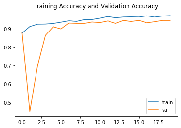
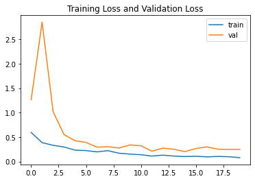
Well, we have great results. Let’s see its graph
Performance Graph
Accuracy Graph
plt.plot(resnet_history.history["acc"],label="train")
plt.plot(resnet_history.history["val_acc"],label="val")
plt.title("Training Accuracy and Validation Accuracy")
plt.legend()
We have good training and validation accuracy.
Loss
plt.plot(resnet_history.history["loss"],label="train")
plt.plot(resnet_history.history["val_loss"],label="val")
plt.title("Training Loss and Validation Loss")
plt.legend()
And less loss.
Closure
Even, such little data, ResNet50 gave satisfactory results. This was it for this blog. See you in the next blog until then Keep Rolling Keep codding.
NOTE: Photo by visuals on Unsplash
Data is taken from DPHI.
The media shown in this article on Covid Detection using X-Ray are not owned by Analytics Vidhya and are used at the Author’s discretion.


